In Google Sheets, conditional formatting enables you to dynamically highlight entire rows based on specific criteria.
Applying the rule is straightforward when you know the column to search. For instance, you might have date entries in column A and wish to highlight rows where column A contains today’s date.
However, it becomes trickier when you want to search within a range. Imagine having a particular value in columns A, B, C, D, or any other column within the range, and you want to highlight the rows containing that value.
In this tutorial, we’ll explore both scenarios, and I’ll also share an interesting tip involving VLOOKUP. VLOOKUP allows you to search down a criterion in a column, return a value from another column, and then highlight the entire row by evaluating the returned value with comparison operators.
Highlighting Entire Rows by Searching for a Key in a Specific Column in Google Sheets
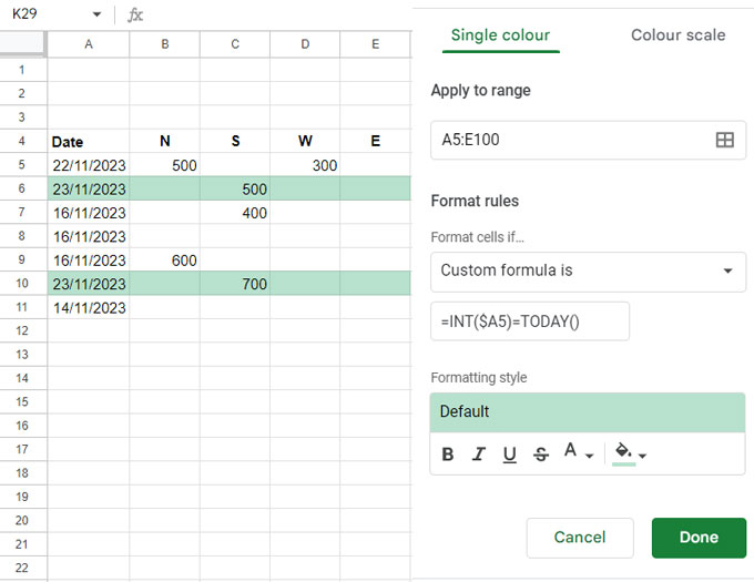
In the following example, the goal is to highlight rows in the range A5:E100 where A5:A100 matches today’s date. How can this be achieved?
- Navigate to cell A1 in the sheet where you want to apply the highlighting.
- Click on Format > Conditional formatting.
- In the field below ‘Apply to range,’ enter A5:E100.
- Select ‘Custom formula is’ from the drop-down under ‘Format rules.’
- Enter the custom formula rule
=INT($A5)=TODAY()in the field below ‘Custom formula is.’ - Choose the text and cell fill color of your choice under ‘Formatting style.’
- Click ‘Done.’
The formula will highlight any row containing today’s date or a DateTime that includes today’s date. If multiple cells in column A contain today’s date or timestamp, all those rows will be highlighted.

To specify a specific date, text, or number as the criterion to highlight the entire row, follow the custom formula examples below:
- Specific Date:
=INT($A1)=DATE(year, month, day) - Text:
=$A1="Apple" - Number:
=$A1=100 - Number with Comparison:
=$A1>=100 - Timestamp:
=$A1=DATE(year, month, day)+TIME(hour, minute, second)
In all these formula examples, replace $A1 with the cell address of the first cell in the search column. For example, if you want to apply this rule to the range C2:G10, and the search column is column G, you should use $G2.
Tip: Including Multiple Search Keys for Conditional Formatting
To include multiple search keys, for example, highlight the rows in the range A5:E100 where values in B5:B100 match either “Apple” or “Orange,” use the OR logical operator as follows:
=OR($B5="Apple", $B5="Orange")Searching Criteria Across Columns and Highlighting Entire Rows in Google Sheets
In the above examples, we discussed knowing the column to search for specific keys. But what if you need to search across columns?
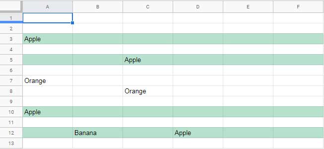
For instance, consider a range to highlight from A1 to Z1000. If you want to highlight rows where any cell in this range contains the string “Apple,” you can use the following formula rule for the ‘Apply to range’ A1:Z1000:
=XMATCH("Apple",$A1:Z1)
The XMATCH function searches for “Apple” across row #1 and returns the column number if found or #N/A if not found. If the result is not #N/A, the rows get highlighted. This automatically applies to each row in the ‘Apply to range’ in conditional formatting.
Highlight an Entire Row Using VLOOKUP in Google Sheets
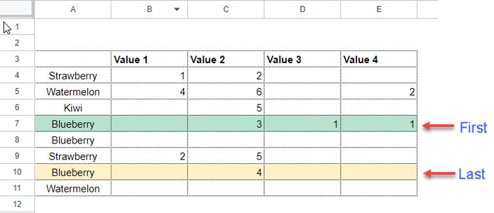
In the following example, my table is in the range A3:E11 where I want to highlight the entire row containing the first occurrence of the fruit “Blueberry” in A3:A11.
In that case, you can use the following VLOOKUP formula for the ‘Apply to range’ A3:E11:
=ROW()=ROW(INDIRECT(CELL("ADDRESS", VLOOKUP("Blueberry", $A$3:$E11, 2, 0))))
Formula Breakdown:
VLOOKUP("Blueberry", $A$3:$E11, 2, 0): This VLOOKUP formula searches for the key “Blueberry” in the cell range $A$3:$E11 and returns the value (result) from the second column in the range. The result column is not important; the range contains 5 columns, so you can specify any column from 2 to 5.- The CELL function returns the cell ID of the result value.
- Wrapping the cell ID with ROW and INDIRECT returns the row number of the VLOOKUP result.
- The rule tests the current row number against the above row number and highlights the matching row.
Note: If you wish to highlight the row of the VLOOKUP result only when the result is a specific value, you can use the following formula:
=AND(VLOOKUP("Blueberry", $A$3:$E11, 2, 0) > 3, ROW() = ROW(INDIRECT(CELL("ADDRESS", VLOOKUP("Blueberry", $A$3:$E11, 2, 0)))))This conditional format rule will be applied only if the result is greater than 3.
How to Highlight an Entire Matching Row from the Bottom of a Table
For the same sample data, you can use the following XLOOKUP formula to highlight an entire row matching a key from the bottom of the table:
=ROW()=ROW(INDIRECT(CELL("ADDRESS", XLOOKUP("Blueberry", $A$3:$A11, $A$3:$A11, , 0, -1))))Here, VLOOKUP has been replaced with XLOOKUP because it can search from the last value to the first value.
The XLOOKUP function searches for “Blueberry” in $A$3:$A11 and returns the value from the same range.
All other formula components remain the same, and so does the logic.
Conclusion
Upon reviewing the formulas, one key observation becomes evident. The use of the dollar sign ($) with cell references is crucial for determining whether they are relative or absolute.
The key principle in highlighting entire rows in Google Sheets is to employ absolute columns and relative rows. When working with a single cell, the column is made absolute, while the row remains relative.
For example: $B5
When specifying a range of cells, the starting cell reference becomes absolute while the ending cell reference becomes column-absolute and row-relative.
For instance: $A$3:$E11
Similar: How to Highlight Vlookup Result Value in Google Sheets.


Is there a way to make it highlight an entire row when certain cells in that row are empty?
I need mine to highlight the row when nothing is in the D and E cells.
Hi, Pine,
This rule would work for you.
=and(NE($D1,""),NE($E1,""))Apply this rule for the whole sheet rows (A1:Z1000) or part of the rows (A1:Z10)
Is there a way to do this with partial text?
I’ve tried the custom formula
=$d2:$d="*apples*"and it isn’t working.Hi, Ryan,
Just use the SEARCH function to do the partial match.
=search("apples",$D2)You aren’t required to use $D2:$D2. Just include the range you want in “Apply to Range.”
Hello, I’d like to use this formula to highlight the entire row whenever there is an error message due to the wrong type of data entered into a cell with a restricted drop-down menu.
Does that make sense?
I tried your formula for highlighting error messages, and that didn’t work, but perhaps that was because they are scattered all over.
Hi, Tara Benavides,
You didn’t specify the cell or column to check for duplicates. I assume it’s column C.
Select all the rows or up to the row you want in your Sheet. Insert the below custom rule in Conditional formatting.
=iserror($C1)Hello,
I am trying to adapt your idea to highlight the entire row into highlighting the entire column instead.
Using your formula:
=ArrayFormula(mmult(n(if($A1:1="Apple",1)),sequence(columns($A1:1),1)^0))but I can’t manage.
Would you have any idea?
Hi, Francois,
That seems simple.
Apply to range A1:Z
Rule:
=countif(A$1:A,"apple")What is the formula to be able to highlight any row, when I click on any cell?
Hi, Deborah,
Sorry, I don’t think we can do that using a formula. I am unaware of any AppScript, though.