To get the headers of the first non-blank cell in each row, we can use an array or non-array formulas in Google Sheets.
Why should one find the headers or field labels of the first non-blank cell in each row?
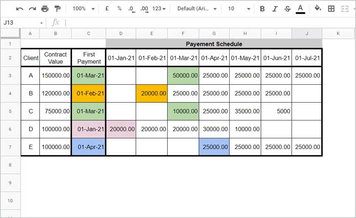
Let’s consider a payment schedule/break-up of a few contracts.
Assume I have signed contracts with five clients, and I have entered their payment schedule in one of my Google Sheets.
Please find the example below (except column C).

The data is arranged similarly to a pivot table.
I want to find the first payment date of each client from the schedule. For that, I have used formula(s) in column C.
To get that, we have to find the headers of the first non-blank cell in each row in the range D3:J7.
Here is how to do that.
Drag-Down Formula to Get the Headers of the First Non-blank Cell in Each Row
In cell C3, insert the following formula.
=index($D$2:$J$2,MATCH(FALSE,ISBLANK(D3:J3),0))Then copy it and paste it into the range C4:C7.
How does this formula find and return the header of the first non-blank cell in a row?
Formula Explanatioin (Non-Array)
1. The MATCH part of the formula finds the relative position of the first non-blank cell in the range D3:J3.
I have detailed the same within one of my earlier tutorials, and that link you can find after a few paragraphs below.
As a side note, the relative position is the count of cells from a starting cell to a target cell (here) horizontally.
Regarding the range D3:J3, the starting cell is D3, and the target cell is F3.
2. The INDEX offsets that many cells (Match output) in the range in the header, i.e., in $D$2:$J$2.
When we drag the C3 formula down, the header range (Index reference) remains the same because we have used absolute reference (dollar signs).
But it returns a different relative position in each row as the reference in the Match, i.e., D3:J3 is relative (without dollar signs).
Related:- Google Sheets: How to Return First Non-blank Value in a Row or Column.
Array Formula to Get the Headers of the First Non-blank Cell in Each Row
We can’t convert the above Index and Match combination as an array formula that expands down.
It’s because the Match will only accept a single row or column reference.
But that doesn’t limit a Google Sheets user from writing an array formula to get the headers of the first non-blank cell in each row.
How?
Please follow the below steps and formula explanation.
Steps
1. Empty the range C3:C7.
2. Enter the following array formula in cell C3, and voila!
=index(
     sortn(
        query(
           split(
              flatten(ROW(D3:J7)&"|"&D2:J2&"|"&D3:J7),
              "|"
           ),
           "Select * where Col3 is not null"
        ),
        9^9,2,1,1
     ),
     0,2
)
How does the above formula return the header of the first non-blank cell in each row in Google Sheets?
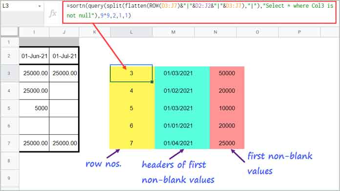
What I have done is – A) unpivot the table range D3:J7, B) filter out blank value cells and C) delete duplicate rows.
I’ll explain that below.
Formula Explanation (Array)
We must peel the formula or take out FLATTEN, SPLIT, QUERY, SORTN, and INDEX parts from it and test them individually.
When testing each part, except SORTN and INDEX, I may additionally use the ARRAYFORMULA function. Otherwise, they won’t work in standalone use.
A) Unpivot Data:
1. FLATTEN
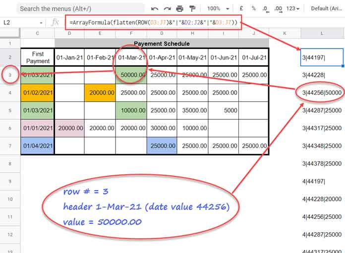
=ArrayFormula(flatten(ROW(D3:J7)&"|"&D2:J2&"|"&D3:J7))I have combined row numbers and headers with every value in the range in the following syntax.
Syntax: row_number|header|value
If any cell in the range is blank, the formula may only return row_number|header|
Please see this.

2. SPLIT
=ArrayFormula(split(flatten(ROW(D3:J7)&"|"&D2:J2&"|"&D3:J7),"|"))In this step, we will separate the row numbers, headers, and values into separate columns.
We have unpivoted the data!
B) Filter Out Blank Value Rows:
3. QUERY
=ArrayFormula(query(split(flatten(ROW(D3:J7)&"|"&D2:J2&"|"&D3:J7),"|"),"Select * where Col3 is not null"))The Query filter out rows that has blank values, or we can say keep row_number|header|value and omit row_number|header|
C) Delete Duplicate Rows:
For the below tests the ARRAYFORMULA is not required.
4. SORTN
Here it removes duplicates based on a selected column, and that is column contains row numbers.
=sortn(query(split(flatten(ROW(D3:J7)&"|"&D2:J2&"|"&D3:J7),"|"),"Select * where Col3 is not null"),9^9,2,1,1)
5. In the final formula, I have used INDEX to extract the second column.
Conclusion
When you use an array formula to get the headers of the first non-blank cell in each row in Google Sheets, you must make sure one thing.
What’s that?
There must be at least one value in each row.
As per the above example, there must be at least one payment in the range D3:J7 in each row.
That’s all. Thanks for the stay. Enjoy!
Resources:
- Get the Header of the Last Non-blank Cell in a Row in Google Sheets.
- Lookup and Retrieve the Column Header in Google Sheets.
- Find Max N Values in a Row and Return Headers in Google Sheets.
- Search Across Columns and Return the Header in Google Sheets.
- Hlookup to Search Entire Table and Find the Header in Google Sheets.
- Filter Values Between Two Group Headers (Titles) in Google Sheets.
- Column Header of Max Value in Google Sheets Using Array Formula.
- How to Retrieve Column Header of Min Value in Google Sheets.


