The FV function in Google Sheets is all about calculating the future value of a periodic investment at a fixed interest rate. By using this function, you can also find the future return of a lump-sum payment.
The fact is, many of us aren’t well-versed in manual financial calculations. So, it’s better to depend on a spreadsheet application for such purposes. Luckily, financial functions are built into tools like Google Sheets and Excel.
Since Google Sheets is cloud-based and free to use, it’s a good idea to learn some of its financial functions. It will really help you stay financially disciplined. In this tutorial, I’ll show you how to use the FV function in Google Sheets with practical examples.
The Syntax of the FV Function in Google Sheets
I’ve already covered the purpose of the FV function above. Now let’s dive into its syntax and how it works.
FV(rate, number_of_periods, payment_amount, [present_value], [end_or_beginning])Arguments:
- Rate: This is the interest rate per period. If you enter the interest rate in a cell (say, Cell C4), you can reference it in different ways.
For example, if the annual interest rate is 5%, you can enter it as5%,0.05, or even5and then useUNARY_PERCENT(C4)in the formula. - Number of Periods (Nper): The total number of payment periods.
- Payment Amount (Pmt): The payment made in each period. If you’re calculating the FV of a lump-sum investment, this can be 0, but then you must provide the
present_value. - Present Value (Pv): Optional. Defaults to 0. If omitted,
Pmtmust be included. Pv represents the current value of the investment. - Type: Optional. Indicates when payments are due:
0for the end of the period (default), and1for the beginning.
Important: Enter both Pmt and Pv as negative values, since they represent cash outflows.
Formula Examples of the FV Function in Google Sheets
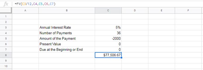
1. Future Value (FV) with Monthly Payments
To calculate the FV of an investment, you need three inputs: the interest rate, the total number of periods, and the payment amount.
Let’s say you invest $2,000 per month for 3 years at a 5% annual interest rate.
=FV(5%/12, 3*12, -2000)Result: $77,506.67
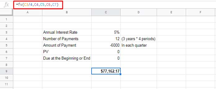
2. Future Value (FV) with Quarterly Payments
If you don’t earn a monthly salary, quarterly investments might be more manageable. For example, let’s say you invest $6,000 every quarter (equal to 3 × $2,000 monthly) over 3 years at an annual interest rate of 5%.
=FV(5%/4, 12, -6000)Result: $77,162.17
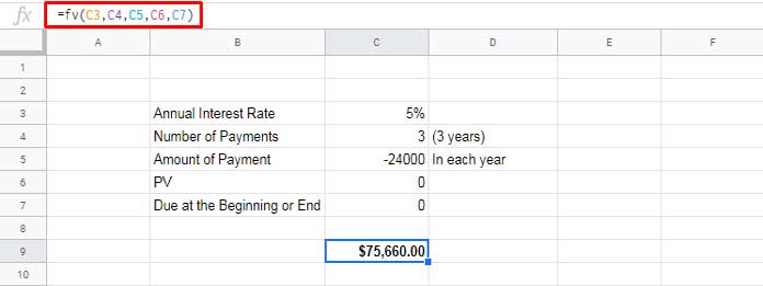
3. How to Use the FV Function in Yearly Payments
If your payments are annual, you don’t need to divide the interest rate. Keep it as is.
=FV(5%, 3, -24000)Result: $75,660.00
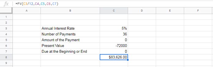
FV Function in Google Sheets to Calculate Lump-Sum Future Value
While the FV function is commonly used for periodic payments, it also works for lump-sum investments. As mentioned earlier, you can use the FV function in Google Sheets to calculate the future value of a one-time payment.
Example:
- Interest Rate: 5% annually
- Periods: 36 months (3 years)
- Present Value: $72,000
=FV(5%/12, 36, 0, -72000, 0)Result: $83,626.00
Comparison of Future Values
Let’s summarize the future values for different payment methods:
- Monthly: $77,506.67
- Quarterly: $77,162.17
- Yearly: $75,660.00
- Lump-sum: $83,626.00
The differences in the future values are primarily due to compounding frequency. Generally, the more frequently interest is compounded (monthly vs. quarterly vs. yearly), the higher the return. Also, a lump-sum investment grows faster because the entire amount starts compounding from day one—unlike periodic investments where only part of the money is invested initially.
What Can You Learn from This?
If you invest a total of $72,000 (either all at once or through periodic payments) for 3 years at 5% interest, the final return will vary based on the payment method.
So, depending on your financial situation, you can choose the investment method that works best for you.
This is just one example of how to use the FV function in Google Sheets to make informed investment decisions. Explore further, and let the FV function help you take control of your finances!


