


It’s almost impossible to extract total and grand total rows from a Pivot table report using the GETPIVOTDATA function in Google Sheets. But there is an alternative formula.
Of course, to dynamically pull aggregated values from a Pivot table, including from a total row, you can use the GETPIVOTDATA function.
But with this function, you can’t pull an entire total row without nesting it.
For example, see the below nested GETPIVOTDATA formula in cell E12 and the pivot table report in A1:D12.
={"Grand Total",GETPIVOTDATA("Sum of Total Sales",A1),GETPIVOTDATA("Average of Total Sales",A1)}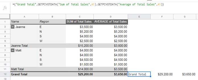
The formula successfully extracts the grand total row.
But what about including the subtotal rows? I mean the “Jeanne Total” and “Matt Total” rows.
The GETPIVOTDATA nested formula will become very complicated. Please see the example below.
={"Jeanne Total",GETPIVOTDATA("Sum of Total Sales",A1,"Name","Jeanne"),GETPIVOTDATA("Average of Total Sales",A1,"Name","Jeanne");{"Matt Total",GETPIVOTDATA("Sum of Total Sales",A1,"Name","Matt"),GETPIVOTDATA("Average of Total Sales",A1,"Name","Matt")};{"Grand Total",GETPIVOTDATA("Sum of Total Sales",A1),GETPIVOTDATA("Average of Total Sales",A1)}}You can ignore this formula. You can’t call this a dynamic formula because, for each total row, you must nest the formula.
That means you can’t use the GETPIVOTDATA function dynamically to extract the individual totals and grand total rows from a Pivot table.
Instead, you can use a FILTER + SEARCH combo, which is dynamic.
When the source changes, the total rows may move up or down. My formula is ready to accommodate those changes.
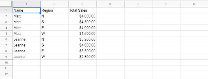
Let’s consider a small dataset (sales report of two employees).
Here are the Pivot table settings used to generate the above Pivot table report.
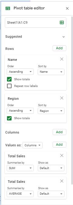
As a side note, to access the Pivot table editor, go to the Insert menu Pivot table.
Formula to Extract the Total Rows From a Pivot Table Report in Google Sheets
The following Filter + Search combo will pull the subtotal and total rows from the above Pivot table.
=filter(A1:D,search("Total",A1:A)>1)It’s a very clean formula compared to the GETPIVOTDATA one above. It’s also dynamic.
Formula Output:
| Jeanne Total | $15,200.00 | $3,800.00 |
| Matt Total | $14,000.00 | $3,500.00 |
| Grand Total | $29,200.00 | $3,650.00 |
Why should I call it dynamic?
For example, assume you have added one more employee to your sales report.
The formula will include that person’s total also in the extracted output.
How to Use the Filter + Search Combo in Pivot Table to Pull Data
The FILTER function is handy to use to filter a table with conditions. You can use this function in a Pivot table too.
FILTER(range, condition1, [condition2, ...])I have used the Search formula to feed the Filter criterion/condition1. It is because I want to do a partial match.
I want to filter rows in the Pivot table column A that contain the string ‘Total.’
That’s why I have used the Search function within Filter.
The Search function will return a numeric number if the string ‘Total’ is available in a row. So the criterion will be;
search("Total",A1:A)>1Some of you may ask about the possibility of using any wildcard characters within the Filter. The answer is NO. That’s why I have used the Search function.
That’s all about extracting total rows dynamically from a Pivot table in Google Sheets.
I hope you have enjoyed this tutorial. See you next time with another Google Sheets tutorial.
Similar Tutorials:
- Create an Age Analysis Report Using Google Sheet Pivot Table.
- Month Wise Pivot Table Report in Google Sheets Using Date Column.
- Group Dates in Pivot Table in Google Sheets (Month, Quarter, and Year).
- Adding Calculated Field in Pivot Table in Google Sheets.
- Drill Down in Pivot Table in Google Sheets (Date Field).
- How to Sort Pivot Table Grand Total Columns in Google Sheets.
- How to Sort Pivot Table Columns in the Custom Order in Google Sheets.