Do functions like Vlookup, Sumif, etc. scare you? Don’t worry. Try the Explore feature in Google Sheets. It may not help you to learn the functions but can solve your problems associated with.
Explore is a small button on the bottom right corner of your Google Sheets window. Clicking on it will open a sidebar panel. Also, you can access it quickly using the Alt+Shift+X shortcut key.
The purpose of Explore in Google Sheets is to help you solve your Google Sheets problems. Type your question and get custom formula or chart suggestions instantly.
The Explore feature in Google Sheets is useful not only for beginners but also for its regular users. Quite recently I myself have used the Explore feature to create a Scatter chart, which normally was plotting a wrong trendline. I have detailed that tips here – Common Errors That You May Face in Scatter Chart in Google Sheets.
Basic row formatting and Charts are also the part of this Google Sheets ‘Assitant’. Below I am trying to explain how to use the Explore feature in Google Sheets.
How to Ask Questions in Explore in Google Sheets
Just typing any question is not a good practice in Explore. Your questions should be phrased in a way the Explore can analyze. I am trying to train you how to ask well-phrased questions in the Explore panel.
If you have a well-arranged data, you can use Google Sheets Explore feature to get formula suggestions. In order to get proper answers, you must include column heading or field label in your Question. I will explain that below.
Must Read: Column Heading | Column Label | Column Name | Field | Field Label in Google Sheets.
When you ask questions to the Explore, the Google Sheets’ ‘Assistant’ (I wish to call it an assistant), the formula that you may get may not be the one you are expecting.
Suppose when you want to look up a value, the formula you are expecting from the Explore may be Vlookup. But you may get a different formula but with the correct answer!
This is because we can use different formulas to solve the same problem due to the versatility of functions in Google Spreadsheets. A Vlookup can be replaced by a Sum + Unique + Filter combination, Index and Match combo, Indirect and Match, or with even a Query.
Get Formulas Generated Using Explore Feature in Google Sheets
I am trying to get answers to some of the problems that can normally be solved by using, Sum, Count, Average, Sumif, Vlookup, Filter like functions.
Again I am telling you the formula suggested by the Explore may contain a different function or function combination but the result would be probably correct. The correctness that we can check manually though.
Sum/Count/Average with the Help of Sheets Explore Feature
Examples:
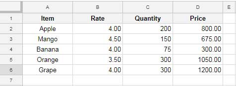
Suppose I want to sum the “Price” column. Ask the question as below.
Your Question should be phrased like “sum Price” or “sum Column D”.
How?
Open the Explore panel by hitting the Alt+Shift+X shortcut. Type either of the above questions as below.
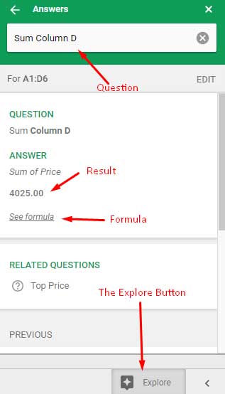
Click See formula link and copy the formula and paste in cell D7. Here is the Explore recommended formula that I got.
=SUM(Sheet12!D2:D6)
To Count “Item”, type the question “Count Item”. To find the average rate and get the formula, type the question “Average Rate”.
Note: To manually learn all the popular Google Docs Sheets functions, please check my Google Sheets Functions Guide.
Vlookup Using Explore Feature in Google Sheets
When I don’t have a demo data to test formulas, I normally depend on fruits data as the sample. So that even though the data is not realistic, it would be better to learn formulas and experiment with it.
In the below fruits data, see how to find the Price of the item “Banana” using Vlookup. The Vlookup formula in cell G2 returns the price.

How does the Explore feature in Google Docs Sheets come handy here?
If you are not familiar with using Vlookup or unsure which function you should use to look up and find, then you can use the Explore feature in Google Sheets.
Understand the Explore Panel in Google Spreadsheet
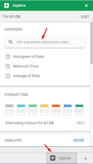
Back to Vlookup (vertical lookup) using Explore.
Click the Explore button to open the sidebar Explore panel. In the field saying “Ask a question about your data” type your question as below.
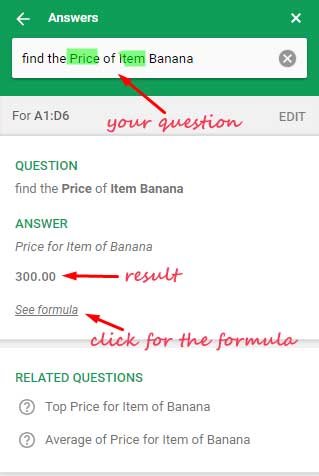
In the question, I have included the field labels “Price” and “Item”. Click the See formula option to get the formula and copy that to your Spreadsheet.
=UNIQUE(FILTER(Sheet12!D2:D6,TO_TEXT(Sheet12!A2:A6)="Banana",Sheet12!D2:D6<>""))
Instead of the Vlookup, the Explore feature in Google Sheets uses a different formula. But the result is the same and that matters the most, right?
Can I phrase the above question differently?
Yes! But use it intelligently. You can use “Item Banana value from Column D” to get the same above result. I mean you must include either the field label or the column heading alphabet in your question.
Sumif/Sumifs Using the Explore Feature in Google Sheets
How to sum a column conditionally with the help of Explore? For example, in the above sample data, I want to sum column D (Quantity) if the date in Column A (Date) is 04/11/2018.
Ask the question “sum of Quantity if Date is 04/11/2018” in the Explore’s designated field. In this question, the “Quantity” and “Date” are the filed labels. As already mentioned you can replace them with Column A and Column D respectively.
Google Sheets Explore feature will probably recommend you the below formula which would return the correct answer of 1683.00.
Formula:
=SUM(FILTER(Sheet12!D2:D10,TO_TEXT(Sheet12!A2:A10)="04/11/2018"))
Of course, this’s not Sumif which is the correct function that we normally use for conditional Sum.
Here is the SUMIF formula that returns the same result.
=sumif(A2:A10,date(2018,11,4),D2:D10)
I found that the Explore in Google Sheets uses the function Filter most often. If Google can tune that, no doubt newbies can use Explore feature in Google Sheets to learn functions. At least they can understand which function is suitable to solve the problem they have in hand.
What about Sumifs in Explore?
I want to deal with multiple conditions in the Sum.
Explore Question: Sum of “Quantity” if “Date” is 04/11/2018 and “Item” is Item 1. There are two conditions and Sumifs is the suitable function.
Here is the formula that returned by Explore which would return the correct result.
=SUM(FILTER(Sheet12!D2:D10,TO_TEXT(Sheet12!A2:A10)="04/11/2018",TO_TEXT(Sheet12!B2:B10)="Item 1"))
Here is the actual Sumifs formula which is more simple and elegant.
=sumifs(D2:D10,A2:A10,date(2018,11,4),B2:B10,"Item 1")
Maxifs Via Google Sheets Explore Feature
Finally, see the normal conditional Max formula and result.
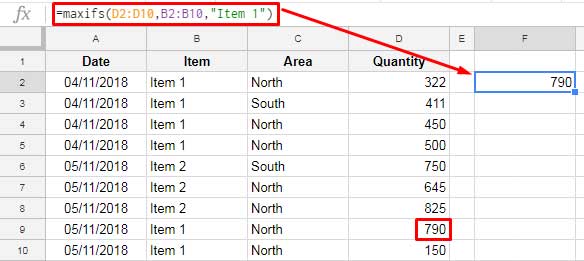
The formula finds the Max value in column D if the “Item” in column B is “Item 1”.
Ask the below question in Explore to get an equivalent formula.
Question: Max Quantity if Item is Item 1.
=MAX(FILTER(Sheet12!D2:D10,TO_TEXT(Sheet12!B2:B10)="Item 1"))
I am concluding the formula part here. You can similarly ask questions to get formula suggestions by Google Sheets.
Personally, I don’t recommend you to use this Explore feature. Of course, it may return the correct result. But if you want to learn functions and code complex formulas by your own, the better way is learning the basic and develop your skills by Googling.
Explore and Alternating Cell Color in Google Sheets
With the help of the Google Sheets explore feature you can add and remove alternating cell color.
Select the table and go to the Explore panel. Scroll down to see the Formatting and click the color you want. Edit and if you don’t like delete it from the same panel later.
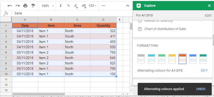
The same is available under the Format menu in Google Sheets.
Chart Suggestion Using Explore
Creating charts are not rocket science in Google Sheets. Have a well-formatted data? Then Google Sheets will do the rest. How?
Just highlight the data and hit Alt+Shit+X. See the chart suggestions. If you can’t find proper chart suggestions don’t hesitate to check my collection of Chart tutorials. You can start it from here – Google Sheets Charts: Built-in Charts, Dynamic Charts, and Custom Charts.
That’s all about the Explore feature in Google Sheets. Hope you have enjoyed the stay.

