Highlight Upcoming Birthdays in Google Sheets

When highlighting upcoming birthdays in Google Sheets, one important aspect is ignoring the year component. For example, if a person’s DOB is 25/12/2010 and today’s date is 22/12/2024, their upcoming birthday is 25/12/2024.

If you have basic knowledge of using the DATE functions in Sheets, you would extract the day and month from the date of birth (DOB) and the year from today’s date, and then join them to make a new date. You can then compare that date with today’s date to determine whether it falls within the specified number of days from today.

However, this approach may fail in certain scenarios. For example, if today’s date is 22/12/2024 and you want to highlight upcoming birthdays in the next 30 days, it could break in some cases.

If the DOB is 15/01/2010, the birthday would be 15/01/2025. So, when you extract the year from today’s date and the other components from the DOB, it becomes 15/01/2024. This means the approach described earlier won’t work.

Here is the correct way to highlight upcoming birthdays in Google Sheets:

Formula:

=LET(
   ref, A1, 
   n, 30, 
   new_dt, DATE(YEAR(TODAY()), MONTH(DATEVALUE(ref)), DAY(ref)), 
   new_dt_adj, IFERROR(IF(new_dt<TODAY(), EDATE(new_dt, 12), new_dt)), 
   ISBETWEEN(new_dt_adj, TODAY(), TODAY()+n, FALSE)
)

You can use this formula to highlight cell A1 for birthdays that fall in the next 30 days, excluding today’s date. Below is an example of how to use this formula in a cell or range, while also controlling the number of days (30 in this case).

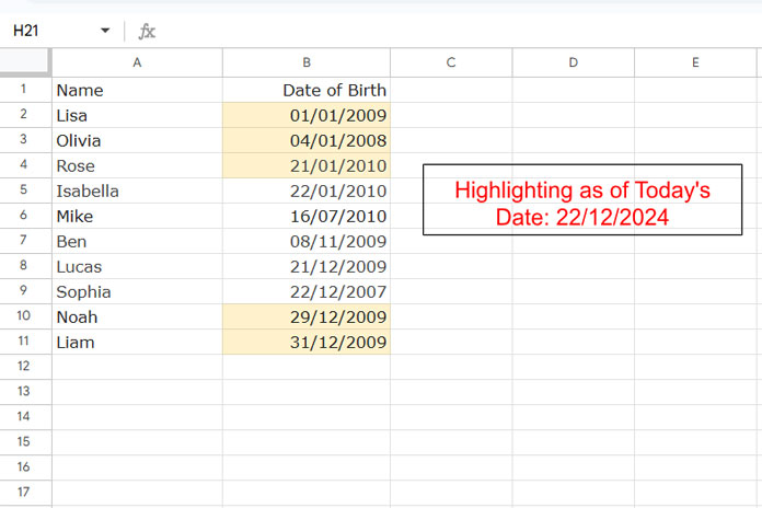
Example of Highlighting Upcoming Birthdays in Google Sheets:

We have the sample data in A1:B, with names in A1:A and DOB in B1:B. The first row contains the field labels.

Sample Data and Highlighting of Upcoming Birthdays in 30 Days

To highlight the dates, follow these steps:

Select the range B2:B.
Click Format > Conditional Formatting.
Choose a fill color under “Formatting Style,” such as light yellow.
Under Format Rules, select Custom Formula Is.
Enter the following formula in the given field and click OK.

=LET(
   ref, B2, 
   n, 30, 
   new_dt, DATE(YEAR(TODAY()), MONTH(DATEVALUE(ref)), DAY(ref)), 
   new_dt_adj, IFERROR(IF(new_dt<TODAY(), EDATE(new_dt, 12), new_dt)), 
   ISBETWEEN(new_dt_adj, TODAY(), TODAY()+n, FALSE)
)

When using a different range (e.g., C5:C100), replace B2 in the formula with the first cell reference in the highlight range (i.e., C5).

The formula highlights upcoming birthdays within the next 30 days. You can replace 30 in the formula with the number of days you want (e.g., 7, 14, 60, etc.).

The formula counts the number of days excluding today’s date, so birthdays that fall today won’t be highlighted. If you want to include today’s birthdays, remove the FALSE in the last part of the formula.

Formula Explanation

The formula may seem complex at first, but it’s quite simple once you break it down. There are three key parts in the formula:

DATE(YEAR(TODAY()), MONTH(DATEVALUE(ref)), DAY(ref)): The DATE function is used in the format DATE(year, month, day), where the year is extracted from today’s date, and the day and month are taken from the DOB itself. The LET function assigns the name new_dt to this value, so it can be reused elsewhere in the formula.
The purpose of the DATEVALUE function is to ensure that the formula returns errors for blank cells instead of a default value like 12/31
IFERROR(IF(new_dt<TODAY(), EDATE(new_dt, 12), new_dt)): The IF function checks whether new_dt is less than today. If true, it advances the date to the same date next year. Otherwise, it returns the same date. This ensures the formula converts all DOBs to dates greater than or equal to today. The LET function assigns the name new_dt_adj to this value.
ISBETWEEN(new_dt_adj, TODAY(), TODAY()+n, FALSE): This tests whether new_dt_adj falls between today’s date and today’s date plus n days (in this case, 30). The conditional formatting highlights cells wherever the formula returns TRUE.

That’s the correct way to highlight upcoming birthdays in Google Sheets!

Resources

Want to explore more? Discover additional conditional formatting techniques—from simple rules to advanced formula-based approaches—in the Ultimate Guide to Conditional Formatting in Google Sheets, where all related tutorials are organized in one place.