If you handle employee-related matters in your office, you might need to determine the age of employees based on their birthdates. In this tutorial, you will learn both non-array and array formulas for calculating age from birthdates (DOB) in Google Sheets.

Calculating Age from Birthdates: Years Only

If cell A1 contains the date of birth, for example, 31/12/2000, you can use the following formula to calculate the age in years:

=DATEDIF(A1, TODAY(), "Y")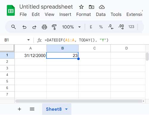

This formula follows the syntax of DATEDIF(start_date, end_date, unit), where start_date is the date of birth in cell A1, end_date is today’s date, and unit is “Y,” representing the number of whole years between start_date and end_date.

The above formula is commonly used to find age from the date of birth (DOB) in Google Sheets.

Ref.: How to Utilise Google Sheets Date Functions [Complete Guide]

Extracting Years from DOB in a Column

If you have dates in column A and want to extract the age, you can use the above formula in cell B1 and drag the fill handle of cell B1 down (copy-paste the formula down).

But you can use an array formula as well which will spill the results down.

=ArrayFormula(IFERROR(DATEDIF(DATEVALUE(A1:A), TODAY(), "Y")))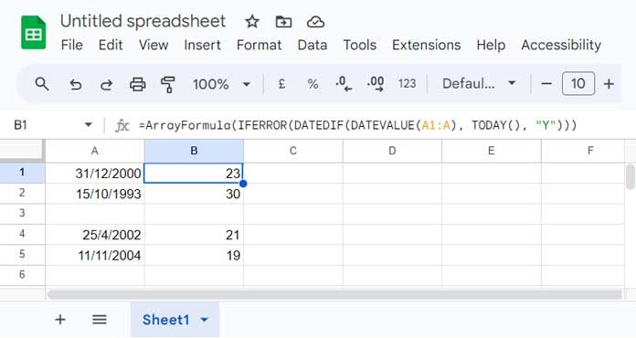

This covers the whole column. But you can limit the expansion up to a specific number of rows by replacing A1:A with a range like A1:A100.

The above is an array formula to return age from the date of birth in Google Sheets.

You may wonder why I don’t simply use:

=ArrayFormula(DATEDIF(A1:A, TODAY(), "Y"))

The reason is it will consider blank cells as 0, which is equal to the date 30/12/1899. So it returns the difference between 30/12/1899 and today’s date.

The DATEVALUE function converts valid dates to date values and returns errors in all other cells. The IFERROR function removes those errors after age calculation.

Calculating Full Age in Years, Months, and Days in Google Sheets

To calculate full age, you need to extract the years, months, and days from the date of birth. We can use the DATEDIF function for that.

Assume the DOB is in cell A1. The following formula will return the age in years, months, and days in three individual cells:

=ArrayFormula(DATEDIF(A1, TODAY(), {"Y", "YM", "MD"}))

The unit in the DATEDIF function contains multiple units such as an array {"Y","YM", "MD"}. So I used the ArrayFormula function.

Where:

• Y: the number of whole years between DOB and today’s date.
• YM: the number of whole months between DOB and today’s date after subtracting whole years.
• MD: the number of days between DOB and today’s date after subtracting whole months.

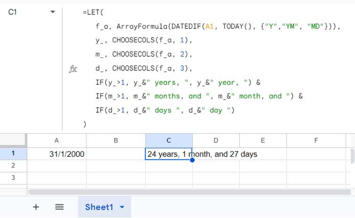
If you want it in the format “n years, n months, and n days“, use the following formula:

=LET(
   f_a, ArrayFormula(DATEDIF(A1, TODAY(), {"Y","YM", "MD"})), 
   y_, CHOOSECOLS(f_a, 1), 
   m_, CHOOSECOLS(f_a, 2), 
   d_, CHOOSECOLS(f_a, 3), 
   IF(y_>1, y_&" years, ", y_&" year, ") & 
   IF(m_>1, m_&" months, and ", m_&" month, and ") & 
   IF(d_>1, d_&" days ", d_&" day ")
)

Formula Explanation:

The formula ArrayFormula(DATEDIF(A1, TODAY(), {"Y","YM", "MD"})) returns the age in years, months, and days in individual cells (an array result). We use the LET function to name it as f_a.

The CHOOSECOLS function extracts the years, months, and days from f_a, and their assigned names are y_, m_, and d_, respectively, using LET.

The IF function evaluates whether the results are a single year, month, or day and assigns the texts “year” or “years”, “month” or “months”, and “day” or “days” accordingly. It then combines the corresponding values (y_, m_, d_) with these texts. Each evaluation is combined, resulting in the final result.

Extracting Full Age from DOB in a Column

To get the years, months, and days in three separate columns, use this formula:

=ArrayFormula(IFERROR(DATEDIF(DATEVALUE(A1:A), TODAY(), {"Y", "YM", "MD"})))

If you enter it in cell B1, it will extract the age in years, months, and days from the range A1:A and spill the results into columns B, C, and D.

If you want it in combined form, use this one:

=ArrayFormula(LET(
   f_a, DATEDIF(A1:A, TODAY(), {"Y","YM", "MD"}), 
   y_, CHOOSECOLS(f_a, 1), 
   m_, CHOOSECOLS(f_a, 2), 
   d_, CHOOSECOLS(f_a, 3), 
   dob, 
   IF(y_>1, y_&" years, ", y_&" year, ") & 
   IF(m_>1, m_&" months, and ", m_&" month, and ") & 
   IF(d_>1, d_&" days ", d_&" day "),
   IF(A1:A="", , DOB)
))

Resources

• How to Sort by Date of Birth in Google Sheets (Formula Options)
• AGE_CALC – A Named Function to Calculate Age or Duration in Google Sheets