Exact Match Using Regular Expression in Google Sheets

This post explains how to perform exact matches for single or multiple strings using regular expressions in Google Sheets.

Note: By “exact match,” we mean the entire cell content must match the pattern exactly — no partial matches. Case sensitivity, however, depends on the function used (e.g., REGEXMATCH is case-sensitive unless modified with a flag like (?i)).

I’ve touched on this topic in earlier tutorials, but those posts had different focal points. Since exact matching with regular expressions may come up in future tutorials, I decided to create this standalone guide so I can link to it when needed. This post is the result of that idea.

There are two primary functions in Google Sheets that support regular expression matching: REGEXMATCH and QUERY.

Though REGEXREPLACE and REGEXEXTRACT also use regular expressions, they aren’t required for exact match operations.

Table of Contents

Functions That Support Exact Match with Regular Expressions

You can use REGEXMATCH to return TRUE or FALSE for an exact match, or use QUERY to filter a range based on exact matches.

Note: Similar to QUERY, you can also use the FILTER function along with REGEXMATCH to filter exact match strings. However, QUERY has the added benefit of aggregation capabilities.

Let’s use the following sample data to demonstrate our formulas:

Sample Data Range: A1:B

Product	Delivery
Product 1	Jan
Product 2	Feb
Product 6	Jan
Product 11	Mar
Product 22	Feb
Products 1 & 5	Feb
Products 2 & 6	Mar

Exact Match with REGEXMATCH in Google Sheets

Single Criterion (Condition)

To test if cell A2 contains “Product 1”, use:

=REGEXMATCH(A2, "^Product 1$")

This returns TRUE only if the cell content matches exactly “Product 1″—it will not match “Product” or “Product 11”.

Note on Case Sensitivity:
By default, REGEXMATCH is case-sensitive. So "Product 1" will not match "product 1".

To make it case-insensitive, use the (?i) flag at the start of your pattern:

=REGEXMATCH(A2, "(?i)^Product 1$")

Use this only when you want to ignore case while matching.

To apply this to an entire column:

=ArrayFormula(REGEXMATCH(A2:A, "^Product 1$"))

But to prevent expanding into blank rows, wrap it with an IF and LEN:

=ArrayFormula(IF(LEN(A2:A)=0, , REGEXMATCH(A2:A, "^Product 1$")))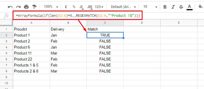

ArrayFormula with REGEXMATCH for exact match using regular expression in Google Sheets

Alternative version:

=ArrayFormula(IF(A2:A="", , REGEXMATCH(A2:A, "^Product 1$")))

Using a Cell Reference for the Criterion

If your criterion is in cell D1, update the formula:

=ArrayFormula(IF(LEN(A2:A)=0, , REGEXMATCH(A2:A, "^" & D1 & "$")))

Multiple Criteria (Conditions)

To match multiple exact values:

=ArrayFormula(IF(LEN(A2:A)=0, , REGEXMATCH(A2:A, "^Product 1$|^Product 22$|^Product 2$")))

If you want to make this multiple-condition match case-insensitive, just add the (?i) flag at the beginning of the pattern:

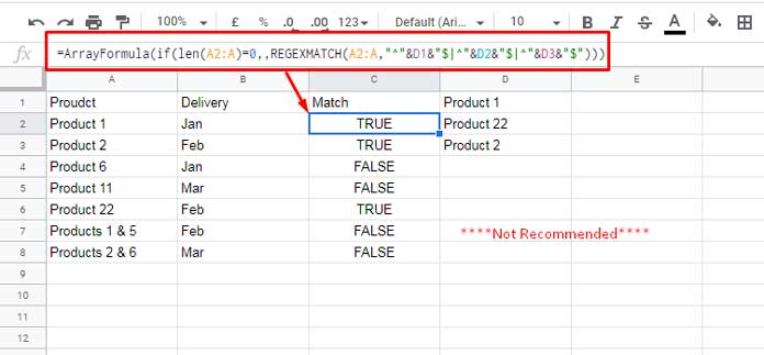
=ArrayFormula(IF(LEN(A2:A)=0, , REGEXMATCH(A2:A, "(?i)^Product 1$|^Product 22$|^Product 2$")))

Using cell references (e.g., D1:D3):

=ArrayFormula(IF(LEN(A2:A)=0, , REGEXMATCH(A2:A, "^" & D1 & "$|^" & D2 & "$|^" & D3 & "$")))

This works but is not flexible, especially if you later add more conditions.

REGEXMATCH pattern matching multiple exact criteria in a Google Sheets column

A more scalable version:

="^" & TEXTJOIN("$|^", TRUE, D1:D) & "$" // case-sensitive
="(?i)^" & TEXTJOIN("$|^", TRUE, D1:D) & "$" // case-insensitive

Use this inside the formula.

Case-sensitive:

=ArrayFormula(IF(LEN(A2:A)=0, , REGEXMATCH(A2:A, "^" & TEXTJOIN("$|^", TRUE, D1:D) & "$")))

Case-insensitive:

=ArrayFormula(IF(LEN(A2:A)=0, , REGEXMATCH(A2:A, "(?i)^" & TEXTJOIN("$|^", TRUE, D1:D) & "$")))

This way, you can maintain flexibility and control whether or not the match is case-sensitive — just by switching the pattern prefix.

Filter Exact Match Using FILTER and REGEXMATCH in Google Sheets

Once you understand the exact match pattern with REGEXMATCH, applying it with FILTER is straightforward.

Syntax:

FILTER(range, condition)

Example:

=FILTER(A2:B, REGEXMATCH(A2:A, "^" & TEXTJOIN("$|^", TRUE, D1:D) & "$"))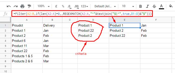

FILTER function with REGEXMATCH to extract exact match rows in Google Sheets

You don’t need to wrap the condition with ARRAYFORMULA here, since FILTER automatically handles arrays.

Exact Match with Regular Expressions in QUERY

If your goal is to filter or aggregate data using exact matches, QUERY is a better fit.

Use the MATCHES operator in the WHERE clause of a QUERY to apply regular expressions for both single and multiple criteria.

Single Criterion

=QUERY(A2:B, "SELECT A, B WHERE A MATCHES 'Product 1'")

If the criterion is in D1:

=QUERY(A2:B, "SELECT A, B WHERE A MATCHES '" & D1 & "'")

Just like REGEXMATCH, QUERY’s MATCHES operator is case-sensitive.

If you want a case-insensitive comparison, use LOWER() on both sides:

=QUERY(A2:B, "SELECT A, B WHERE LOWER(A) MATCHES '" & LOWER(D1) & "'")

Multiple Criteria

You can hardcode values:

=QUERY(A1:B, "SELECT A, B WHERE A MATCHES 'Product 1|Product 22|Product 2'")

Or use a range with TEXTJOIN:

=QUERY(A1:B, "SELECT A, B WHERE A MATCHES '" & TEXTJOIN("|", TRUE, D1:D) & "'")

If you want the match to be case-insensitive, wrap the column and criteria with LOWER():

=ARRAYFORMULA(QUERY(A1:B, "SELECT A, B WHERE LOWER(A) MATCHES '" & TEXTJOIN("|", TRUE, LOWER(D1:D)) & "'"))

We use ARRAYFORMULA here because LOWER(D1:D) produces an array, which needs to be evaluated before it goes into the query.

Unlike REGEXMATCH, which uses the RE2 engine and requires ^ and $ for full-string matches, the MATCHES operator in QUERY uses a different regular expression engine (PREG-like) that automatically matches the entire cell content. So you don’t need to add anchors when using MATCHES in QUERY.

If you don’t want an exact match:

Use CONTAINS for substring matches (best for 2–3 values)
Use MATCHES for complex or multiple patterns (see: Multiple CONTAINS in WHERE Clause in Google Sheets Query)