Explore the power of dynamic cell references in a Google Sheets Table of Contents for easy navigation and flexibility.

But what exactly is a dynamic cell reference in a table of contents?

When creating a table of contents with links to cells, issues can arise, particularly when inserting rows or columns.

Linking to a cell involves using the URL of a cell obtained by right-clicking on the cell and choosing “View more cell actions” > “Get link to this cell.”

We can then use this URL in the HYPERLINK formula or paste it within the provided field in Insert > Link to create a link to the copied cell.

For example, copy the URL of cell C3 as mentioned above. Then in cell A3, you can use either of the below approaches to link to cell C3:

1. Use the following HYPERLINK formula:

=HYPERLINK("https://docs.google.com/spreadsheets/d/1cJb4k3PHPRov...331&range=C3", "Jump")

Syntax:

HYPERLINK(URL, [link_label])

Where:

• URL is the URL that you copied by right-clicking.
• link_label is the text “Jump”.

2. Type “Jump” in cell A3, click on Insert > Link, paste the URL in the provided field, and click Apply.

Inserting/deleting rows above row #3 or columns to the left of column C will move your original linked cell, but the table of contents item will persistently link to cell C3.

So, how can we make the links in a table of contents dynamic?

Utilizing functions like HYPERLINK, ADDRESS, ROW, and COLUMN in Google Sheets allows us to achieve a dynamic cell reference in a table of contents. In this approach, we won’t be able to use the Insert > Link method; instead, we rely on the HYPERLINK function.

How to Get Dynamic Cell Reference in Table of Contents in Google Sheets

To achieve a dynamic cell reference in a Google Sheets table of contents, follow these tips:

Replace the static cell reference C3 in the URL, as illustrated in the example above, with a dynamic reference using the functions ADDRESS, ROW, and COLUMN.

The existing cell reference is a text string, and it won’t update when you move the source cell. Delete C3 in the last part of the URL and combine the URL with ADDRESS(ROW(C3), COLUMN(C3), 4) as shown below:

=HYPERLINK("https://docs.google.com/spreadsheets/d/1cJb4k3PHPRov...331&range="&ADDRESS(ROW(C3), COLUMN(C3), 4), "Jump")

Syntax:

ADDRESS(row, column, [absolute_relative_mode], [use_a1_notation], [sheet])

Where:

• row: ROW(C3), which is the row number of the cell reference.
• column: COLUMN(C3), which is the column number of the cell reference.
• absolute_relative_mode: 4, which means the row and column are relative.

If you want to link to a different sheet/tab in your table of contents, include the corresponding sheet name in the ROW and COLUMN part of the formula. For example:

ADDRESS(ROW(Jan!C3), COLUMN(Jan!C3), 4)

These adjustments ensure that your table of contents has dynamic links that update correctly even if you move the source cells or reference different sheets.

Creating Dynamic Hyperlinks to Cell Ranges in Google Sheets

If you want to create a HYPERLINK formula that dynamically refers to a range of cells in a table of contents, follow these steps.

I have a total of four sheets in a Google Sheets file named “Sheet1,” “Jan,” “Feb,” and “Mar.”

In Sheet1!B4:B6, I have created a table of contents.

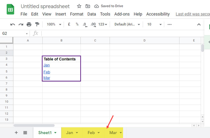
Cell B4, B5, and B6 link to the range B2:C5 in their respective sheets. Here is how to link to a range of cells and make it dynamic.

1. Go to the “Jan” sheet and select the range B2:C5.
2. Right-click and click “View more cell actions” > “Get link to this range.”
3. Use that URL to code a HYPERLINK formula in cell B4 in “Sheet1” as below:

=HYPERLINK("https://docs.google.com/spreadsheets/d/1cJb4k3P...1238YJ0/edit#gid=0&range=B2:C5", "Jan")

However, this formula is not dynamic. Let’s make it a dynamic range reference HYPERLINK formula using the ADDRESS function as earlier.

Remove B2:C5 and combine the below part with the formula.

ADDRESS(ROW(Jan!B2), COLUMN(Jan!B2), 4)&":"&ADDRESS(ROW(Jan!C5), COLUMN(Jan!C5), 4)

Here, we have combined two ADDRESS functions to generate a range reference instead of a cell reference.

The final formula will look as follows.

=HYPERLINK("https://docs.google.com/spreadsheets/d/1cJb4k3P...1238YJ0/edit#gid=0&range="&ADDRESS(ROW(Jan!B2), COLUMN(Jan!B2), 4)&":"&ADDRESS(ROW(Jan!C5), COLUMN(Jan!C5), 4), "Jan")

To dynamically link to other sheets in the table of contents, follow the above steps.

Pros and Cons of Using Dynamic Cell References in Tables of Contents

Pros:

• Single-cell reference: The cell automatically adjusts when you move the source cell by inserting/deleting rows or columns or cut-pasting the cell to a new row/column.
• Cell range: The cell range automatically adjusts when you move the source cell range by inserting/deleting rows or columns or cut-pasting the cell range to a new range.

Cons:

• Single-cell: Nothing notable.
• Cell range: You should take care to move the whole cell range. It may make your dynamic range messy if you only move the first or last cell in the range.