Multi-Row Dynamic Dependent Drop-Down List in Google Sheets

We can create a multi-row dynamic dependent drop-down list in Google Sheets without using Google Apps Script. This tutorial explains how.

I will only use built-in Google Sheets functions to create a multi-row dynamic dependent drop-down list.

Why Dynamic Dependent Drop-Down Lists Are Useful?

Let me explain why a dynamic dependent drop-down list in Google Sheets is a must-try.

Imagine you are running a bookstore. You can create two drop-down lists, one containing all the author names and the other their book titles in a Sheet. Copy them in multiple rows.

When you get inquiries, for example, from educational institutions, you can send them the Sheet via email.

They can select the authors and book titles from the drop-downs and send the file back to you (of course, you can use Google Forms for the same purpose).

There are plenty of such situations where you can use dynamic dependent drop-down lists.

A. Create a Simple Drop-Down List in Google Sheets

Anyone with limited spreadsheet exposure can easily create a simple drop-down list, not dynamic. How?

I must explain this part before starting the tutorial on creating a dynamic dependent drop-down list in Google Sheets because it is the essence of the tutorial.

Your first drop-down menu in Google Sheets is just a click away. To create a simple drop-down list, please do as follows.

A Simple Drop-Down List in Google Sheets

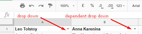
In cell A2, you can see a drop-down list (menu). This drop-down menu allows you to pick any item from the range in C2:C8 from within cell A2.

Steps:

Here the active cell is A2 in “Sheet2.” Go to the menu Data > Data Validation or Insert > Drop-down. Add the rules as per the image below.

Go to Insert > Drop-down and under criteria select Drop-down (from a range) > Enter the range in the field, i.e., Sheet2!C2:C8, and Done.

Our earlier tutorial, Restrict People from Entering Invalid Data on Google Doc Spreadsheet, also shed more light on data validation.

Recommended Reading: The Best Data Validation Examples in Google Sheets.

Now let us move to more complex forms of the drop-down list.

B. How to Create a Dependent Drop-Down List in Google Sheets

To create a dependent drop-down, needless to say, first, there should be a drop-down list. It works like this.

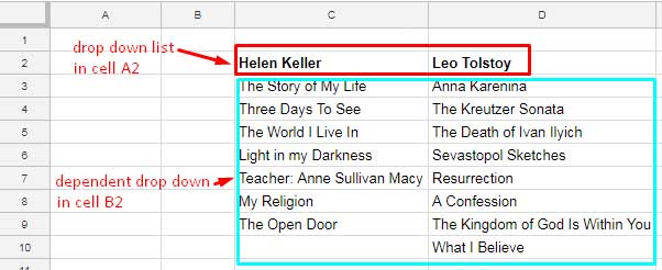
Drop-Down List and Dependent Drop-Down List - Difference

You can see the drop-down list in cell A1 and its dependent in cell B1 in the above screenshot.

You select “Leo Tolstoy” in cell A1. Then all his books will be available to pick in cell B1.

When you pick another author from the list, the list of books in cell B1 should change accordingly.

Now let us learn how to create a dependent drop-down list in Google Sheets.

There are the names of two authors in the range C2:D2. We can use that range to create a drop-down list.

See the list of their books in the range C3:D10 that we can use to create a dependent drop-down list.

We can use the values in cell C2:D2 for the drop-down in cell A2 (Insert > Drop-down > Criteria > Drop-down (from a range) > Sheet2!C2:D2).

In cell B2, we are going to create a dependent drop-down. It’s sometimes called a Dynamic Dependent Drop Down List in Google Sheets.

Here we are using Google Sheets Named Ranges. What is the purpose of Named Ranges in Google Sheets?

With the Named Ranges feature, we can name a range, e.g., C3:C9, to something like sales, total, like any name, and use the same in formulas instead of C3:C9.

Named Range Is Not a Must Here. Then Why Are We Using It?

The main reason is we can use Named Ranges in formulas instead of a range reference.

By doing so, we can make the formulas reader-friendly.

Here we have two authors in the drop-down in cell A2. So we require two named ranges pointing to their book titles.

Create the first named range as below.

Go to the Data menu > Named Ranges and select “Add Range.”

I’ve entered Helen_Keller as the name for the range C3:C9. I’ve used underscore as Named Ranges won’t accept spaces.

Named Range for Dependent Drop-Down in Google Sheets

Similarly above, add another name Leo_Tolstoy for the range D3:D10. So we have two named ranges now!

Formula Part in Google Sheets Dynamic Drop-Down List

We already have a drop-down list in cell A2 (author names).

Now we should write a formula connecting the selected author in it and their book titles. We will write the required formula in cell E2.

Formula:

=if(A2=C2,indirect("Helen_Keller"),Indirect("Leo_Tolstoy"))

I am doing a logical test with Google Sheets IF logical function here.

The formula tests the value in cell A2 with C2.

If it matches, the formula will populate the values from the range C3:C9 (Helen_Keller). If not, it will populate the values from the range D3:D10 (Leo_Tolstoy).

The Named Range requires the Indirect Function to work.

What is the benefit of using the Indirect and Named Range combo here?

It’s equal to the below formula.

=ArrayFormula(if(A2=C2,C3:C9,D3:D9))

With Named Range and Indirect combo, we can avoid using the ArrayFormula. Also, if there are more values to test in the logical part, using an Indirect and Named Range combo can make your formula cleaner.

When you select an item from the drop-down in cell A2, corresponding values will populate in cell E2:E.

Now we can move to the final step, i.e., creating the dependent drop-down list.

To do that, go to the menu Insert > Drop-down > Criteria > Drop-down (from a range) and enter the criteria range E2:E10, and voila! Your dynamic drop-down list in Google Sheets is ready.

Finished Dependent Drop-Down in Google Sheets

From this point, we can create a multi-row dynamic dependent drop-down list in Google Sheets.

We want to modify the formula for this.

C. How to Create a Multi-Row Dynamic Dependent Drop-Down List in Google Sheets

Now let us create a multi-row dynamic drop-down list.

We are following the same steps under Title B. But a few more additional steps are required, which I will explain as and when it comes.

Dynamic Multi Row Dependent Drop-Down List - Sample Data

In cell A1, first, we should create a drop-down list with the author’s name.

To do this, Go to the menu Data > Data Validation > Add rules > Criteria > Drop-down (from a range).

Select the range as C1:F1, which is the authors’ names. (You can do the same from the Insert menu Drop-down also).

Now we have a list of authors as a drop-down in cell A1. From this, we can select any of the four authors.

We need a dependent drop-down list in cell B1 to select the book related to the author in cell A1. Let’s do that part.

Please see a set of Named Ranges for this purpose. If you have doubts about creating it, please scroll up, and see the steps under Title B.

Formula Part in Multi-Row Dynamic Dependent Drop-Down List in Google Sheets

Apply the below formula in Cell G1.

=if(A1=C1,indirect("Agatha_Christie"),if(A1=D1,indirect("Sir_Arthur_Conan_Doyle"),if(A1=E1,indirect("Helen_Keller"),INDIRECT("Leo_Tolstoy"))))

Now in B1, we can create a dynamic dependent drop-down list.

Again, for your info, all the steps are already detailed under Title B above.

Go to B1 and then select the Data menu Data Validation > Add rules > Criteria > Drop-down (from a range). Set the criteria range G1:G15.

Now you can select any author from the drop-down list in cell A1 and the corresponding author’s book from cell B1.

Step 3 - Adding Multi-Row Dynamic Dependent Drop-Down List

Up to here, the steps are similar to that provided under Title B. Now we want the same list in multi-rows.

We are creating a Multi-Row Dynamic Dependent Drop Down List in Google Sheets.

Copying and pasting the drop-down lists in A1 and B1 to the cells down below won’t work.

We should modify the above formula in cell G1 as below.

=ArrayFormula(if(len(A1:A),transpose(if(transpose(A1:A)=C1,indirect("Agatha_Christie"),if(transpose(A1:A)=D1,indirect("Sir_Arthur_Conan_Doyle"),if(transpose(A1:A)=E1,indirect("Helen_Keller"),INDIRECT("Leo_Tolstoy"))))),""))

A Very Important Update on 08-Feb-2023:

You can replace the above complex formula with the below BYROW one.

=byrow(A1:A,lambda(r,ifna(transpose(filter(C2:F,C1:F1=r)))))

This formula doesn’t use INDIRECT so the Named Ranges are also not required.

Now go to cell B1 and modify the data validation range from G1:G15 to G1:T1.

A Very Important Update on 02-Feb-2021:

Please make sure one thing!

You are using absolute cell reference in the A1 and relative cell reference in the B1 criteria range.

To do that, go to Data > Data validation, select the A1 rule, and ensure that the range is $C$1:$F$1, not C1:F1.

Then select the B1 rule and ensure that the range is G1:T1, not $G$1:$T$1.

Now copy and paste the lists (drop-downs) in cells A1 and B1 down the columns as far as you want.

Multi-Row Multi Column Dynamic Dependent Drop-Down List - Final

That’s all.

We have successfully created our first-ever Multi-Row Dynamic Dependent Drop Down List in Google Sheets. I hope you have enjoyed it!

drop_down_sample

Please feel free to make a copy of this sheet, where I’ve done my above experiments.

127 COMMENTS

Martin February 17, 2021 At 2:53 pm

Hi. Sorry to interrupt you. Would you please explain the following two things to me?

len(A1:A),
transpose(A1:A)=C1

What does A1:A mean?
- Prashanth February 18, 2021 At 8:41 am
  
  Hi, Martin,
  
  A1:A is column A which contains the drop-downs. len(A1:A) means non-blank cells in the range A1:A.
  
  The function TRANSPOSE used to change the column orientation (vertical to horizontal).
  - Jaishree August 17, 2021 At 7:00 pm
    
    The question here – If I add a new row to the sheet, here my formulae is going for a toss – how to avoid that?
    - Prashanth August 18, 2021 At 4:44 am
      
      Hi, Jaishree,
      
      I couldn’t reproduce that issue in the example sheet that I included within this tutorial.
Sunil February 17, 2021 At 1:57 am

Hello Prashant,

I tried everything as you mentioned post the update but when it comes to mentioning ='Sheet1'!$H$16:$K$16 in the Data range under Data validation (C1:F1 as per your example), when I click save, there is a red error box appears and it says “Please enter a valid range”.

Could you please help here because only the first cell works (A1 for you and D3 for me) but when I copy and paste further below, nothing shows up in (B2, your example)?

Could you please help?

Thanks,
Sunil
- Sunil February 17, 2021 At 2:09 am
  
  In your example of B1 > Data > Data Validation > enter data range > here the system is not accepting when I type ='Sheet1'!G1:T1. It says “Please enter a valid range”.
  
  Please help.
  
  Thanks,
  Sunil
  - Prashanth February 17, 2021 At 8:47 am
    
    Hi, Sunil,
    
    Please make sure you spelled the sheet name correctly.
    
    Also, you can check my example sheet for the same.
    - Sunil February 17, 2021 At 1:35 pm
      
      Hi Prashant,
      
      Yes, I’ve spelled it correctly, and also checked your example sheet, which very clearly has the data range starting from = and also accepts the $ value prefixed to the cells. When I do the same, the error message is “Please enter a valid range”.
      
      I’ve spent hours just re-entering the data validation range in multiple options, but it never worked.
      
      Please do help me.
      
      Thanks,
      Sunil
      - Prashanth February 17, 2021 At 2:07 pm
        
        Hi, Sunil,
        
        It’s actually a new Google Sheets feature. I think it’s not yet rolled out fully. So please wait a few more days.
Rachel February 8, 2021 At 9:17 am

Hi,

I have managed to do all the formulas. My only problem is copying B1 downwards. The list range does not automatically copy. I have about 1000 rows.
- Prashanth February 8, 2021 At 10:56 am
  
  Hi, Rachel,
  
  Earlier there was the issue. Now the drop-down supports relative reference.
  
  In B1, the data validation “List from a range” must be =G1:T1, not =$G$1:$T$1.
  
  When you copy down you will see the copied drop-down flagged. Just delete the values by selecting B2:B1000.
  
  Related – Relative Reference in Drop-Down Menu in Google Sheets.
Raju January 12, 2021 At 2:18 am

Hello Prashanth,

Following is the link to the sheet.

… link copied and then removed by the admin …

Would like your help in resolving this issue I’m facing.

I have managed to get data validated in the same row depending on the selection of cell A1. But I would like to get it vertically.

Eg.: Cell B2 has (rooms)
Need B3 to give dynamic data validation depending on the room type selected in B2.
- Prashanth January 15, 2021 At 9:20 am
  
  Hi, Raju,
  
  I have gone through your sheet to understand your requirement. You want the drop-down and the dependent drop-down in the same column.
  
  My solution won’t be able to fulfill your requirement as the formula in G1 populates the dependent drop-down values (B1:B drop-down) based on the values in column A (A1:A drop-down).
OM Kumar Chaurasiya January 8, 2021 At 2:33 pm

When I drag the validation column to below, dependent data validation not dynamically changed. There is needed one by one data validation.

I need an entire column, could you please help me.
- Prashanth January 8, 2021 At 2:54 pm
  
  Hi, OM Kumar Chaurasiya,
  
  You may require to use Apps Script. Please go thru’ the comments to find the relevant link.
- Prashanth February 2, 2021 At 12:01 pm
  
  Hi, OM Kumar Chaurasiya,
  
  It changes now. Thanks, Google for the update.
  
  You may please check my tutorial once again to see the update.
Manorma RANA July 16, 2020 At 10:55 am

Hi Prashanth,

I have used your formula for 10 column data. I have added values accordingly but the formula works only for 4 columns.

I’m getting the error “Wrong number of arguments to IF. Expected between 2 and 3 arguments, but received 4 arguments.”

Can you help?
- Prashanth July 18, 2020 At 9:41 am
  
  Sheet URL (with edit access) please.
Tricia Curran May 15, 2020 At 4:04 am

Thanks for this! The only issue I’m currently having is that I get #N/As appearing in my dropdown list because the lists are shorter. Is there a way to avoid this? Thanks in advance.
- Prashanth May 15, 2020 At 10:40 am
  
  Use IFNA() to remove the N/A errors from the data validation range. I haven’t seen that issue in my test.
Onyx May 8, 2019 At 4:14 am

Thanks for this! It was quite helpful, and while a little clunky, it allowed me to do exactly what I needed to do. Nevermind manually changing 200 cells…it is still much better than the alternatives.
- Prashanth February 2, 2021 At 11:59 am
  
  Hi, Onyx,
  
  Now, no need to manually change the rows. I have updated the tutorial based on the lastest Google Sheets program changes.
Bo April 20, 2019 At 12:22 am

How can I add a third column? A dependent list for the first dependent list?
Kelly April 19, 2019 At 5:31 pm

Thank you so much, I used your example and was able to create a basic work order for our flooring business. One question that I have, how can I now connect the options to a price in a third column? For example Author > Title > Price. I would love to do that but my understanding of sheets and excel is limited.
- Prashanth April 19, 2019 At 10:02 pm
  
  Hi, Kelly,
  
  You can maintain a price list in another tab and use Vlookup. If you can share a copy (just demo data) of your Sheet, I may be able to help you.
  
  Best,
j April 15, 2019 At 12:45 am

My multiple dropdowns work, as long as I do not sort. If I want to sort alphabetically then the data validation gets messed up. Suggestions?
- Prashanth April 15, 2019 At 11:48 am
  
  Hi,
  
  Open a new tab and use the SORT formula.
  
  =sort(Sheet1!A1:B,1,true,2,true)
  
  If you want you can filter the author too.
  
  =filter(Sheet1!A1:B,Sheet1!A1:A="Helen Keller")
  
  Best,
  
  Prashanth KV
Chris March 15, 2019 At 2:59 am

“This’s because while copy and pastes a data validation list, there is no option in Google Sheets to change the range automatically.”

I’m working with more than 3k+ data points. It’s literally faster to just have my team type in the data for themselves. If there is an actual way of creating dependent dropdowns I would love to hear it.
- Prashanth March 15, 2019 At 4:07 pm
  
  Hi, Chris,
  
  Sorry for the inconvenience.
  
  If you have several rows of data, you must depend on a script.
- Prashanth February 2, 2021 At 11:58 am
  
  Hi, Chris,
  
  Here is a good news. Google has added the capability. Based on that I have updated my tutorial. Please go through it again.
amaury March 7, 2019 At 8:45 pm

Hello, Thanks for that.

Do you have it with 4 dependent dropdown column?

Regards,

Amaury
- Prashanth March 8, 2019 At 11:11 am
  
  Hi, Amaury,
  
  You can do that by following my tutorial. I don’t have a template for that now.
James March 6, 2019 At 7:34 pm

Hello Prashanth,

I did a similar project 3 years ago on March 2, 2016….

https://docs.google.com/spreadsheets/d/1q9ZTWGiJvDgk6RTuWffXbtAGGGf7sBZsIo2GlPaMYwY/copy

TC James/mreighties 🙂
- Prashanth March 7, 2019 At 9:40 am
  
  Hi, James,
  
  Welcome!
  
  It’s a different approach and good too. It also serves the purpose.
Aziz February 25, 2019 At 7:49 pm

I have a problem, i want to make a multiple dropdown list but it’s don’t work.

Can you help me ?