The COUPDAYS function in Google Sheets helps you determine the number of days in the coupon period (interest payment period) that contains the settlement date.

If you’re unfamiliar with the term “settlement date,” don’t worry! It’s explained in detail in the Arguments section below. Scroll down to learn more.

Before diving into how to use the COUPDAYS function, let’s first clarify the term “coupon”, which will help you understand the function better.

What Is a Coupon?

For first-time bond investors, the term “coupon” can be confusing. In simple terms, it refers to the annual interest payment that the bondholder receives from the bond’s issue date until it matures.

In the past, investors who purchased bonds were given physical certificates that had a series of attached coupons (scheduled interest payments). While these physical coupons are no longer used, the term “coupon” has stuck.

For example, if you have a $1,000 bond with a 6% coupon, it will pay $60 annually. If the payment frequency is semiannual (twice a year), the bondholder will receive $30 twice a year.

As a side note, if you want to find the number of coupon payments, you can use the COUPNUM function. The arguments for both the COUPNUM and COUPDAYS functions are the same.

COUPDAYS Function in Google Sheets: Syntax and Arguments

Syntax:

COUPDAYS(settlement, maturity, frequency, [day_count_convention])

Arguments:

• settlement – The settlement date of the security (bond). This is the date after issuance when the bond is traded to the buyer.
• maturity – The maturity or expiry date of the bond.
• frequency – The number of coupon payments per year (annual, semiannual, or quarterly).
• day_count_convention – This optional argument specifies the method used for counting days in the coupon period.
  Available options:
  • 0 – US 30/360 (30-day months and 360-day years as per NASD standards)
  • 1 – Actual/Actual (commonly used for non-financial purposes)
  • 2 – Actual/360
  • 3 – Actual/365
  • 4 – European 30/360 (follows European conventions for 30-day months and 360-day years)

Example of COUPDAYS Function in Google Sheets

Let’s explore how to use the COUPDAYS function with cell references.

In this example, you’ll use the settlement date, maturity date, frequency, and day count convention as inputs.

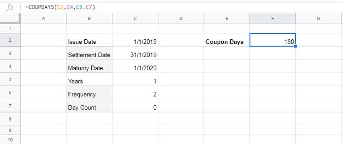
Formula:

=COUPDAYS(C3, C4, C6, C7)

Here, the COUPDAYS formula in Cell F2 returns the number of coupon days as 180. Now, if you change the frequency in Cell C6 to 1, the formula will return 360 days.

This means:

• A frequency of 1 corresponds to 360 days (annual payments),
• A frequency of 2 gives 180 days (semiannual payments),
• A frequency of 4 gives 90 days (quarterly payments).

If you change the day count convention from 0 to 1, the results will be 365 days, 181 days, and 90 days respectively, reflecting a different method of counting days.

In summary, the day count convention plays a crucial role in calculating coupon days using the COUPDAYS function in Google Sheets.

Using COUPDAYS with Input Values Directly

If you’re entering values directly in the COUPDAYS function, use the DATE function to input the settlement and maturity dates.

For example, if your settlement date is 31/1/2019 and your maturity date is 1/1/2020, you must enter them as:

DATE(2019, 1, 31)

and

DATE(2020, 1, 1)

Even if your dates are formatted as mm/dd/yyyy, you still need to use the DATE function in this format.

Common Errors in the COUPDAYS Function

There are two common errors you might encounter when using the COUPDAYS function in Google Sheets: #VALUE! and #NUM!.

Causes of Errors:

• #VALUE! error occurs when you input invalid dates.
• #NUM! error is caused by:
  • Using out-of-range values for the frequency or day count convention.
  • Having the settlement date greater than or equal to the maturity date.

That’s all you need to know about the COUPDAYS function in Google Sheets! Hope this guide helps you effectively use the function. Enjoy!