")
")


")


")

")
")
 in Excel & Google Sheets")


This tutorial explains how to use COUNTIFS with ISBETWEEN in Google Sheets. Along the way, you’ll also see how to combine them with other matching criteria.
Let’s start with a simple example.
Suppose you want to know how many times you filled fuel in your vehicle during a given period.
Normally, in COUNTIFS you’d use comparison operators (>=, <=, etc.) to check if dates fall within your start and end dates. But with ISBETWEEN, you can simplify that process and avoid common mistakes.
Why Use ISBETWEEN with COUNTIFS?
When working with COUNTIFS, comparison operators must be wrapped inside quotation marks (like ">="&D2). This is easy to overlook—especially since functions like FILTER don’t require that.
Instead of using operators like >, >=, <, <=, you can directly use ISBETWEEN with COUNTIF or COUNTIFS.
This makes your formulas easier to read and less error-prone.
In short: COUNTIFS + ISBETWEEN is ideal when you want to count values that fall between two dates or numbers—along with one or more additional criteria.
COUNTIFS with ISBETWEEN: Syntax
COUNTIFS Function:
COUNTIFS(criteria_range1, criterion1, [criteria_range2, criterion2], …)When using ISBETWEEN, the structure changes a bit.
- Normally, we place operators in the criterion part.
- With ISBETWEEN, the test itself goes in the criteria_range part.
- The criterion becomes simply
TRUE.
Example 1: COUNTIFS Between Two Dates
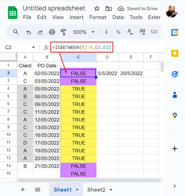
In the example below, column A contains Client Names and column B contains PO Dates.
We want to count the number of POs between a start date in cell D2 and an end date in E2.
Formula:
=COUNTIFS(ISBETWEEN(B2:B, D2, E2), TRUE)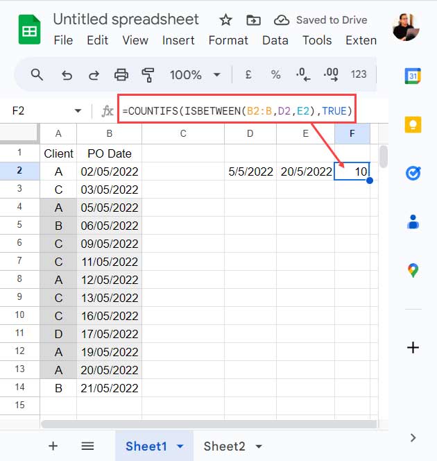
Here:
criteria_range1→ISBETWEEN(B2:B, D2, E2)criterion1→TRUE
How It Works
The ISBETWEEN function checks if each PO date falls between the start and end dates.
It returns TRUE or FALSE.
Then COUNTIFS counts how many TRUE values there are.
If you don’t want the boundary dates included, specify FALSE to exclude the boundary dates:
=COUNTIFS(ISBETWEEN(B2:B, D2, E2, FALSE, FALSE), TRUE)Example 2: COUNTIFS Between Two Dates + Matching Criteria
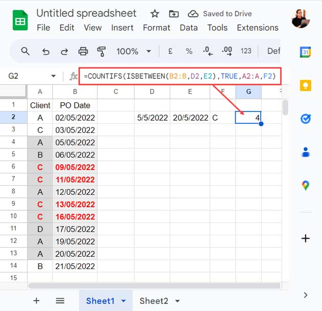
Using the same dataset (Client names in column A, PO dates in column B):
- Start date → D2
- End date → E2
- Client name → F2 (say “C”)
Formula:
=COUNTIFS(ISBETWEEN(B2:B, D2, E2), TRUE, A2:A, F2)This counts how many POs came from client C between 05/05/2022 and 20/05/2022.
Multiple Criteria Example
What if you want to count POs from clients “A” and “D” in the same date range?
=ARRAYFORMULA(SUM(COUNTIFS(ISBETWEEN(B2:B, D2, E2), TRUE, A2:A, {F2, F3})))Here:
{F2, F3}is an array of client names inside curly brackets.SUMcombines the counts.- ARRAYFORMULA helps process it correctly.
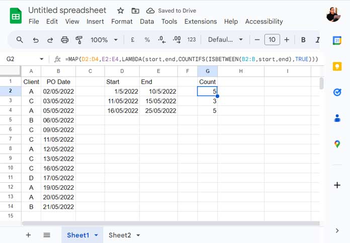
COUNTIFS with ISBETWEEN and Multiple Date Ranges
There are two ways to handle multiple sets of start and end dates:
- Drag-down method – Lock ranges with
$and copy the formula down.
Example: ReplaceB2:Bwith$B$2:$Bbefore dragging. - Spill-down method (using MAP + LAMBDA) – A cleaner, array-friendly approach.
Formula with MAP:
=MAP(D2:D4, E2:E4, LAMBDA(start, end, COUNTIFS(ISBETWEEN(B2:B, start, end), TRUE)))This spills the results for each start–end pair.
You can also add criteria like client names:
=MAP(D2:D4, E2:E4, F2:F4, LAMBDA(start, end, client, COUNTIFS(ISBETWEEN(B2:B, start, end), TRUE, A2:A, client)))If you want to use open ranges such as D2:D and E2:E instead of D2:D4 and E2:E4, wrap them with TOCOL to remove blank cells.
Example:
=MAP(TOCOL(D2:D, 1), TOCOL(E2:E, 1), LAMBDA(start, end, COUNTIFS(ISBETWEEN(B2:B, start, end), TRUE)))Conclusion
Using COUNTIFS with ISBETWEEN makes your formulas simpler and reduces the chances of errors with comparison operators.
- Use it to count values between two dates or numbers.
- Combine it with one or more criteria.
- Extend it with MAP + LAMBDA for multiple ranges.
If you face any issues, first try the examples exactly as shown here. Once they work, adapt them to your own dataset.
Have a question? Drop it in the comments, and I’ll get back to you ASAP.