You can use the following formula to count the number of rows between two values in Google Sheets:

=ROWS(XLOOKUP(value1, range, range):XLOOKUP(value2, range, range)) - 2

When using this formula, replace value1 with the first value to look up in the column and value2 with the second value to look up.

Then, replace range with the column range reference.

Count Specific Entries Between Two Values in Google Sheets

If you want to count specific values between two values, use this formula:

=COUNTIF(OFFSET(XLOOKUP(value1, lookup_range, count_range), 1, 0):OFFSET(XLOOKUP(value2, lookup_range, count_range), -1, 0), criterion)

Where:

• value1 – The first value to look up
• value2 – The second value to look up
• lookup_range – The range to search for the values
• count_range – The corresponding range to count from
• criterion – The specific value to count

Example: Counting Rows Between Two Values in Google Sheets

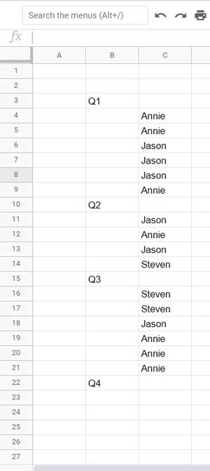
In the following example, I want to count the number of rows between the strings “Q1” and “Q2” in column B (range B2:B1000).

Formula:

=ROWS(XLOOKUP("Q1", B2:B1000, B2:B1000):XLOOKUP("Q2", B2:B1000, B2:B1000)) - 2

The formula would return 6, which is the number of rows between the specified two values.

How the Formula Works

• XLOOKUP("Q1", B2:B1000, B2:B1000) – Matches the first value and returns its reference.
• XLOOKUP("Q2", B2:B1000, B2:B1000) – Matches the second value and returns its reference.
• XLOOKUP("Q1", B2:B1000, B2:B1000):XLOOKUP("Q2", B2:B1000, B2:B1000) – Creates a range from the first to the second value.
• ROWS(...) returns the number of rows in this range, including both values. Since we only need rows between these values, we subtract 2 from the result.

That’s the easiest way to count the number of rows between two values in Google Sheets.

Example: Counting Specific Entries Between Two Values in Google Sheets

In the above example, how do we count how many times the name “Annie” appears between the two values in another column?

Formula:

=COUNTIF(OFFSET(XLOOKUP("Q1", B2:B, C2:C), 1, 0):OFFSET(XLOOKUP("Q2", B2:B, C2:C), -1, 0), "Annie")

This formula will return 3, as there are three cells containing “Annie” between “Q1” and “Q2” in column C.

How the Formula Works

• OFFSET(XLOOKUP("Q1", B2:B, C2:C), 1, 0) – XLOOKUP finds “Q1,” and OFFSET moves one row down.
• OFFSET(XLOOKUP("Q2", B2:B, C2:C), -1, 0) – XLOOKUP finds “Q2,” and OFFSET moves one row up.
• OFFSET(XLOOKUP("Q1", B2:B, C2:C), 1, 0):OFFSET(XLOOKUP("Q2", B2:B, C2:C), -1, 0) – Defines the range between “Q1” and “Q2,” excluding them.
• COUNTIF(...) counts the occurrences of “Annie” within this range.

That’s how to count a specific entry between two values in Google Sheets.

Where Does This Apply in Real Life?

These formulas are useful for identifying values between two reference points in a column. They work with dates, numbers, and text, but they are especially useful for text-based filtering. This allows you to find all values between two labels and manipulate the data—count, average, sum, etc.—with ease.

Resources

• How to Count Values Between Two Dates in Google Sheets
• Lookup a Date Between Two Dates in Google Sheets
• Filter Values Between Two Headings in Google Sheets
• Excel Formula to Extract All Rows Between Two Texts in a Column
• Slicing Data with XLOOKUP in Google Sheets