


")


")

")
")
 in Excel & Google Sheets")


If you merge cells, only the top-left cell in the merged range retains the value — the rest become blank. This behavior stays the same when you copy and paste those cells. So how do you copy-paste merged cells without blank rows in Google Sheets?
Without copy-paste commands, transferring data through a computer interface wouldn’t be as easy as we think. On Windows, you can use Ctrl+C to copy and Ctrl+V to paste. On a Mac, just replace Ctrl with the Command key.
In Google Sheets, we can use these commands to get things done ASAP. I’m not downplaying the importance of the Cut command either — it’s just as useful.
Besides the basic copy-paste options, there’s also a special one in Google Sheets: Paste special. I’ll come back to that in a second.
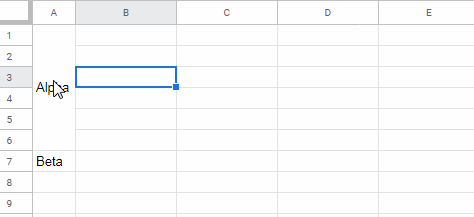
There’s no built-in option in Google Sheets to copy-paste merged cells without bringing along blank rows or spaces. If you simply copy and paste, the values appear as is — with all the blanks included.
If you use Paste special (Ctrl+Shift+V), it unmerges the cells and pastes only the values — but the blanks caused by merging remain.
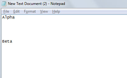
What about pasting those values into another application like Notepad? Check the screenshots below.
- Extra blank rows in the pasted column (column B) in Google Sheets (Screenshot #1).
- Extra spaces when pasted into Notepad (Screenshot #2).
To copy-paste merged cells without blank rows or spaces, try the following approaches.
How to Copy and Paste Merged Cells Without Blank Rows in Sheets
If your goal is just to copy values from a column of merged cells to another column without blank rows in between, use the FILTER formula.
Example (Scenario #1 – Screenshot #1): In cell B1, use this formula:
=FILTER(A1:A, A1:A<>"")This filters out the blank cells — in other words, it extracts only the visible values from column A, ignoring the blanks caused by row merging.
Alternatively, you can use the QUERY function:
=QUERY(A1:A, "SELECT A WHERE A <> ''")How to Copy to Notepad Without Extra Spaces (Scenario #2)
If you’re pasting the merged values into Notepad or another plain text editor, you don’t need any extra steps. Just use the output of the FILTER or QUERY formula and copy it directly — no spaces will be carried over.
Merged Cells to Unmerged – Multiple Columns
What if your merged cells span multiple columns?
You can still use the FILTER formula like this:
=LET(data, VSTACK(A1:A, B1:B), FILTER(data, data<>""))This combines the values from columns A and B (including any merged rows) into a single column in, say, column D.
Want two separate columns instead?
Use the original FILTER formula in cell D1, then drag it to the right to apply it to both columns A and B:
=FILTER(A1:A, A1:A<>"")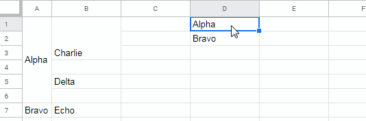
Alternatively, you can use this formula, which does the job in one go:
=BYCOL(A1:B, LAMBDA(col, FILTER(col, col<>"")))This will ‘paste’ the values from each column into adjacent unmerged columns without blank rows — exactly what you want.
Additional Tip
If you merge cells across a row, like A1:Z1, use this formula to get the value only:
=FILTER(A1:Z1, A1:Z1<>"")Note: The results from formulas like FILTER, QUERY, or BYCOL are dynamic. If you change the original (source) data, the formula output will update automatically.
If you want to keep a static version of the result, copy the formula output and paste it as values (Ctrl+Shift+V on Windows or Command+Shift+V on Mac).
That’s all about how to copy-paste merged cells without blank rows in Google Sheets. Thanks for reading — enjoy!
Resources
- Pad Values in Google Sheets for Clean Notepad Pasting
- Uncover Merged Cell Addresses in Google Sheets
- Merge Values from Two Columns into One in Google Sheets
- How to Sort Vertically Merged Cells in Google Sheets
- How to Fill Merged Cells Down or to the Right in Google Sheets
- Sequence Numbering in Merged Cells In Google Sheets
- Filtering When Columns Contain Merged Cells in Google Sheets
- Creating Sequential Dates in Equally Merged Cells in Google Sheets