If you have a date separated by dots that is not recognized as a valid date by the ISDATE function, you may need to convert it before using it for assignments, comparisons, or summarizing by date, month, etc. You can convert text-formatted dates with dots to a slash format, which Google Sheets recognizes as a valid date.

Generic Formula

=LET(seg, SPLIT(A2, "."), DATE(CHOOSECOLS(seg, 3), CHOOSECOLS(seg, 2), CHOOSECOLS(seg, 1)))

Where:

• A2 contains the text-formatted date separated by dots.
• SPLIT(A2, ".") divides the date into day, month, and year components.
• CHOOSECOLS(seg, 3), CHOOSECOLS(seg, 2), CHOOSECOLS(seg, 1) extract the year, month, and day, respectively, to construct a valid date using the DATE function.

The above formula assumes the date in A2 is in dd.mm.yyyy format. If the date follows the yyyy.mm.dd format, use the following formula instead:

=LET(seg, SPLIT(A2, "."), DATE(CHOOSECOLS(seg, 1), CHOOSECOLS(seg, 2), CHOOSECOLS(seg, 3)))

Example of Converting Text Dates with Dots to Slash Format in Google Sheets

Suppose we have text dates separated by dots in column A2:A.

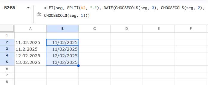
To convert them to a slash-formatted date, use the following formula in cell B2 and drag it down:

=LET(seg, SPLIT(A2, "."), DATE(CHOOSECOLS(seg, 3), CHOOSECOLS(seg, 2), CHOOSECOLS(seg, 1)))

• The SPLIT function splits the text date in A2 using a . (period) as the delimiter.
• The CHOOSECOLS function extracts each segment from the split result and arranges them in the correct order within the DATE function, which follows the syntax: DATE(year, month, day)

The output will be a valid date. If you are not satisfied with the default format, you can modify it by navigating to Format > Number > Custom date and time.

Converting Text Dates with Dots to Slash in a Column

To apply the formula to an entire column, replace A2 with A2:A and enter it as an array formula. However, this may return #VALUE! errors in rows corresponding to empty cells.

You might consider using IFERROR to suppress these errors, but doing so alone will remove the date formatting, returning only date values. To retain the date format, wrap IFERROR with TO_DATE as follows:

=ArrayFormula(TO_DATE(IFERROR(LET(seg, SPLIT(A2:A, "."), DATE(CHOOSECOLS(seg, 3), CHOOSECOLS(seg, 2), CHOOSECOLS(seg, 1))))))

Alternative Formula Using REGEXEXTRACT and DATE Combination

Instead of splitting at a specific delimiter, we can extract the day, month, and year components separately using REGEXEXTRACT:

Regex Patterns:

• ^(\d+)\.: Captures one or more digits before the first dot.
• \.(\d+)\.: Captures one or more digits between two dots.
• \.(\d+)$: Captures one or more digits after the last dot.

So, the formula to convert text-formatted dates with dots to slash format will be:

=DATE(REGEXEXTRACT(A2, "\.(\d+)$"), REGEXEXTRACT(A2, "\.(\d+)\."), REGEXEXTRACT(A2, "^(\d+)\."))

If the date is in yyyy.mm.dd format, use:

=DATE(REGEXEXTRACT(A2, "^(\d+)\."), REGEXEXTRACT(A2, "\.(\d+)\."), REGEXEXTRACT(A2, "\.(\d+)$"))

To apply this formula to an entire column, use:

=ArrayFormula(TO_DATE(IFNA(DATE(REGEXEXTRACT(A2:A, "\.(\d+)$"), REGEXEXTRACT(A2:A, "\.(\d+)\."), REGEXEXTRACT(A2:A, "^(\d+)\.")))))

Explanation:

• IFNA handles empty cells by preventing #N/A errors.
• TO_DATE ensures the output remains in date format.

Resources

• Convert Date to String Using the Long-winded Approach in Google Sheets
• How to Convert Date to Month and Year in Google Sheets
• Convert Dates to Fiscal Quarters in Google Sheets
• Format a Date Without Converting it Into a Text – Google Sheets
• Convert Dates to Week Ranges in Google Sheets (Array Formula)
• Convert Month Name to Days in Google Sheets
• Convert Month Name to Month Number in Google Sheets
• Convert Month Numbers to Month Names in Google Sheets