


")


")

")
")
 in Excel & Google Sheets")


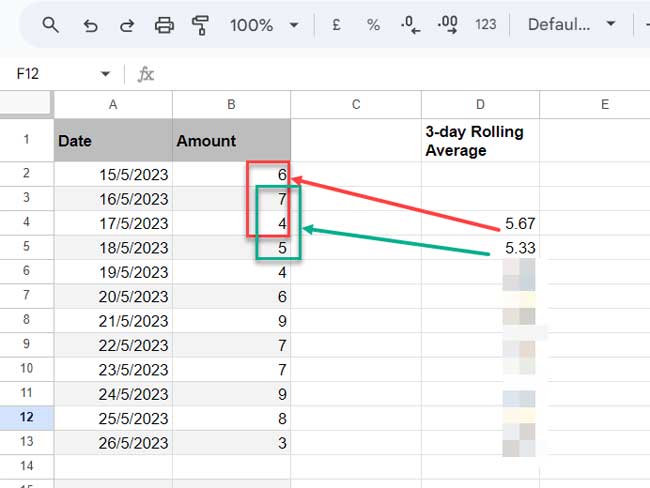
In Google Sheets, calculating a rolling N-period average is a powerful way to analyze trends in time-based data by smoothing short-term fluctuations. Whether you’re tracking sales, web traffic, or any other metric over time, a rolling average helps reveal the underlying pattern more clearly.
In this tutorial, you’ll learn how to calculate a rolling average across a specified number of periods—such as 3-day, 7-day, or 30-day averages—using both drag-down and array formulas. We’ll also show you how to make the formulas dynamic, so they automatically adjust as new data is added.
Note: The terms rolling average and moving average are often used interchangeably in spreadsheets. While they may have subtle distinctions in other contexts, both generally refer to the average of a sliding window of recent values.
If you’re specifically looking for moving average techniques, please check the Related Resources section at the end of this tutorial.
Sample Data
Here’s a sample dataset we’ll use throughout the tutorial:
| Date | Amount |
|---|---|
| 15/5/2023 | 6 |
| 16/5/2023 | 7 |
| 17/5/2023 | 4 |
| 18/5/2023 | 5 |
| 19/5/2023 | 4 |
| 20/5/2023 | 6 |
| 21/5/2023 | 9 |
| 22/5/2023 | 7 |
| 23/5/2023 | 7 |
| 24/5/2023 | 9 |
| 25/5/2023 | 8 |
| 26/5/2023 | 3 |
What Is “N” in a Rolling Average Formula?
In a rolling average, N refers to the window size—the number of data points used to compute each average. For example, a 3-day rolling average uses the current value and the previous two values.
Rolling N Average Using a Drag-Down Formula
Assuming the data is in A1:B, and the values start in B2, here’s how to compute a 3-day rolling average:
Step-by-Step:
- In cell
D4, enter:
=AVERAGE(B2:B4)- Drag this formula down to apply it for all available data.
If you want a 7-day rolling average instead, use this in cell D8:
=AVERAGE(B2:B8)Each result reflects the average of the N most recent values.
Rolling N Average Using a Dynamic Array Formula
To generate a rolling average using a dynamic array formula, use the MAKEARRAY and CHOOSEROWS functions:
Formula (for 3-period average):
=MAKEARRAY(ROWS(B2:B13), 1, LAMBDA(r, c, IFERROR(AVERAGE(CHOOSEROWS(B2:B13, SEQUENCE(3, 1, r-3+1))))))Place this in D2 and it will expand downward.
This version avoids manual dragging and handles errors automatically for the first few rows.
Change the Window Size (N)
To change the rolling average window to, say, 7 days:
- Replace both instances of
3with7.
Optional: Make the Range Open-Ended
To make the formula work with a dynamic data range:
=MAKEARRAY(ARRAYFORMULA(XMATCH(TRUE, B2:B<>"", 0, -1)), 1, LAMBDA(r, c, IFERROR(AVERAGE(CHOOSEROWS(B2:B, SEQUENCE(3, 1, r-3+1))))))This approach auto-detects the number of data points based on non-empty cells.
Understanding the Formula
Let’s break down the array formula:
=MAKEARRAY(ROWS(B2:B13), 1, LAMBDA(r, c, IFERROR(AVERAGE(CHOOSEROWS(B2:B13, SEQUENCE(3, 1, r-3+1))))))MAKEARRAY(...): Creates an array of rows equal to the number of data points.r: Represents the current row index (starting from 1).SEQUENCE(3, 1, r-3+1): Generates a sequence of 3 positions, starting fromr - 3 + 1. For example, whenr = 3(i.e., the 3rd output row, or D4), it returns{1, 2, 3}— corresponding toB2:B4.CHOOSEROWS(B2:B13, ...): Extracts those rows from the data range.AVERAGE(...): Computes the average of the selected 3 values.IFERROR(...): Suppresses errors for the first two rows where insufficient data is available.
Summary
Rolling averages are a great way to smooth time-based data and track underlying trends. In this guide, we covered two practical approaches:
- Drag-down formulas: Best for quick setups when your dataset isn’t too large.
- Array formulas: Ideal when you want the rolling average to update automatically as new values are added.
You can easily adjust the rolling window size (N) by changing a single value in the formula. And if your data grows over time, the dynamic version using XMATCH will ensure your averages stay up to date without manual edits.
Related Resources
- Reset Rolling Averages Across Categories in Google Sheets
- Google Sheets: Rolling Average Excluding Blank Cells and Aligning
- Calculating Running Average in Google Sheets (Array Formulas)
- Calculating Simple Moving Average (SMA) in Google Sheets
- Average Every N Cells with an Array Formula in Google Sheets
- Weighted Moving Average in Google Sheets (Formula Options)
How do you account for the preceding values, excluding empty rows, within the rolling n-average (I’ve figured this part out)? Additionally, how do you ensure that the rolling average array aligns with the placement of nonempty cells?
Hi Jack,
I have alternative formulas, different from the ones mentioned above, which I’ll share once you respond. Have you thought about utilizing a FILTER formula to exclude blank cells from the data before applying the previously mentioned formula?
If you provide more details, I can better understand the actual scenario. Also, I suggest sharing the URL of an example sheet below for more effective assistance.
Hi Jack,
Please check out my new tutorial. You can find the link at the end of the post.