


At present, the Bullet list is not part of the Google Sheets menu. The easiest way to insert bullet points in Google Sheets is by using the CHAR function. Another method is using Custom formatting (recommended).
I recommend the custom formatting based bullet list-making in Google Sheets as it doesn’t involve any physical character at the beginning of the bullet list.
Google Sheets is a Spreadsheet application, not a word processor. So we can’t complain about not having a menu option to insert Bullet Points in it.
That doesn’t mean we are left with no options. As mentioned, there are the CHAR function, custom formatting, and some keyboard shortcuts to insert Bullet Points in Google Sheets.
Now regarding the CHAR function, you may not be new to this. I have used this function earlier to get Subscript/Superscript letters and numbers in Google Sheets.
Here are the workaround to insert white and black (filled and unfilled) bullet points and other essential bullets/symbols in Google Sheets.
I have two approaches – formula as well as custom formatting based approaches.
There is one more approach involving the Alt+ numeric keypad numbers. But that way you can insert only 2-3 bullet points and may not support all the PC.
First I am going to give you all the essential bullet points in Google Sheets. After that, I will explain how to create your bulleted list in Google Spreadsheets using either a formula or custom formatting. For both, you must first know how to get bullet symbols.
How to Get Bullet Symbols in Google Sheets
You can use the below formulas to get all the necessary bullet symbols in Google Sheets. Create it first. Then I will show you how to use it in formulas as well as in custom formatting to create a bullet list.
Essential Bullet Points
| Bullet Name | Formula | Symbol |
| Bullet | =char(9679) | ● |
| White Bullet | =char(9675) | ○ |
| Triangular Bullet | =char(8227) | ‣ |
| Hyphen Bullet | =char(8259) | ⁃ |
| Inverse Bullet | =char(9688) | ◘ |
| Inverse White Bullet | =char(9689) | ◙ |
| Circle White Bullet | =char(9678) | ◎ |
| Circled Bullet | =char(9673) | ◉ |
Star Bullets Points
| Bullet Name | Formula | Symbol |
| Star Bullet | =char(9733) | ★ |
| White Star Bullet | =char(9734) | ☆ |
| Inverse Star Bullet | =char(10026) | ✪ |
Miscellaneous and Most Frequently Using Bullets Points
The below list contains some of the bullets that are most common in use in bulleted lists.
| Bullet Name | Formula | Symbol |
| Flower Symbol | =char(10020) | ✤ |
| Sixteen Pointed Asterisk Symbol | =char(10042) | ✺ |
| Snowflakes Symbol | =char(10052) | ❄ |
| Rotated Heavy Black Heart Symbol | =char(10085) | ❥ |
| Rotated Floral Heart Symbol | =char(10087) | ❧ |
| Hand Symbols | =char(9754) | ☚ |
| =char(9755) | ☛ | |
| =char(9756) | ☜ | |
| =char(9758) | ☞ |
How to Insert Bullet Points in Google Sheets (Formula Approach)
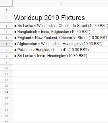
Here, for example, I am inserting the Inverse Bullet symbol in a list. You can find the formula for the same above. It is;
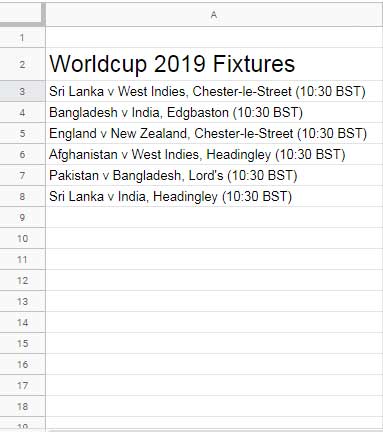
=char(9688)First, prepare your list. For example, here is my list in column A.
Enter the above formula in cell B1 and simply copy the Inverse Bullet output symbol. Then double click the item in your list and paste the symbol at the beginning.
Repeat these steps for each item.
If your list is very large you will find inserting bullet points a time taking process in Google Sheets. So you can use an Array Formula to solve this.
Must Read: Array Formula: How It Differs in Google Sheets and Excel.
Inserting Multiple Bullet Points in Google Sheets
Assume, my list is in A3:A. Then I can use this array formula in cell B3.
=ArrayFormula(if(len(A3:A),char(9688)&" "&A3:A,))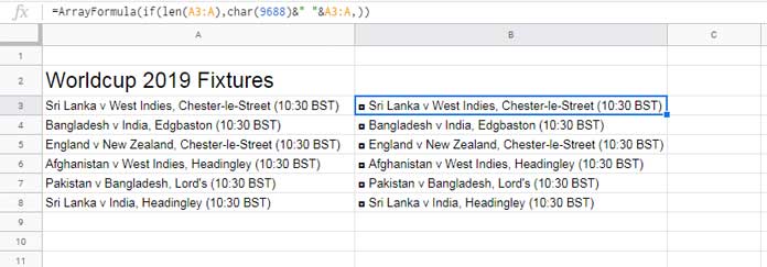
Highlight the range B3:B8 and copy the content. Then right-click on cell A3 and apply, Paste special > Paste values only. Delete the formula in cell B3.
The Disadvantage of this Formula Approach: Since we are physically adding a bullet point character, we will find tough to apply Filtering in the bulleted list.
Custom Formatting and Bullet List in Google Sheets
I have already detailed how to get bullet symbols using the Char formula. We can use that to create a bulleted list.
For example, I want to use the Snowflakes Symbol as the bullet in a list. Here are the step-by-step instructions to use it as the bullet in a list.
Steps to Use Snowflakes Symbol in Custom Formatting for Making a Bulleted List
1. Get the Symbol in a Blank Cell.
For that, enter the formula =char(10052) in any blank cell for example cell G1. Then simply copy the content (symbol) from the Cell using the Ctrl+C or right-click and Copy.
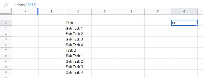
2. Select the Cell to Apply the Bullet.
Select cell C3 first. We want the Snowflakes symbols to apply to the range C3:C6 and C8:C11 (all the sub-tasks). That we can do later with the format painter.
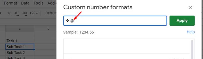
3. Custom Format the Cell C3.
- Go to the menu command Custom number format (Format > Number > More Formats > Custom Number Format).
- In the blank field there paste the snowflakes symbol (Ctrl+V or right-click and Paste).
- Tap the spacebar and then type “@” then click “Apply”. If you want more space between the bullet point and the text, tap the spacebar multiple (2-3) times.
- Click “Apply”.
4. Paint Format.
The active cell is cell C3 in which you have already inserted the Snowflakes bullet symbol. Copy the content and select the range C4:C6, right-click and apply Paste special > Paste format only.
Repeat this step for the range C8:C11. Alternatively, we can use the format painter.
This way you can create a bullet point list without a formula in Google Sheets.
The Advantage of this Custom Format Approach: This method doesn't add any physical characters to the existing list.
That’s all. I hope you have enjoyed this Bullet list tips and tricks in Google Sheets.