The easiest way to create a running total of expenses or other values in Google Sheets is by using a non-array formula. However, you can also achieve this with several array formulas.
For array formulas, you can use functions such as SUMIF, DSUM, MMULT, and SCAN (LAMBDA Helper Function – LHF). In this tutorial, I’ve included formulas based on these functions in addition to a non-array (drag-down) formula.
In real-life scenarios, cumulative sums are widely used. One example is in a cricket match, where the total score is the running sum of the runs scored. Each time a player scores runs, they are added to the total.
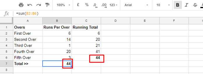
In the screenshot below, column C represents a cumulative sum (CUSUM) in a cricket match.

If you’re unfamiliar with cricket, simply focus on the numbers. The sum of cells B2:B6 (found in B7) matches the value in C6, which is the cumulative sum of runs/numbers in B2:B6.
In C2:C6, you can see the running total of the values in B2:B6.
Running Total with Non-Array Formula
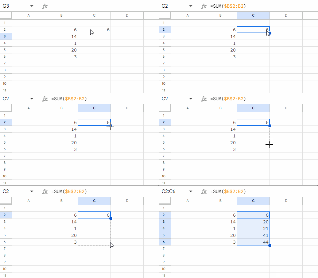
In cell C2, enter the following SUM function:
=SUM($B$2:B2)Once you’re in cell C2, move your mouse to the fill handle at the bottom-right corner of the cell. When the pointer changes to a + sign, click and drag it down to cell C6.

Alternatively, you can enter the formula in cell C2, then copy and paste it into cells C3:C6.
This is the easiest way to calculate a running total using a non-array formula in Google Sheets.
It works because the range in the SUM function expands as you drag it down. This happens because the first part of the range is an absolute reference, while the second part is a relative reference.
Running Total with Array Formulas
Below, you’ll find four array formulas for calculating a running total in Google Sheets, using SUMIF, MMULT, DSUM, and SCAN.
Out of these, I recommend using SUMIF for its simplicity and ease of use. MMULT and DSUM are a bit more complex. While SCAN is also easy to use, it may cause performance issues with large datasets.
I’m including all these options for two reasons:
- You might encounter one of them in a shared sheet.
- To demonstrate how different formula combinations can produce the same result.
Running Total with ARRAYFORMULA, SUMIF, and ROW
We use SUMIF for conditional summation in Google Sheets. This function can also be applied to calculate running totals by using a smart condition, which I’ll explain below.
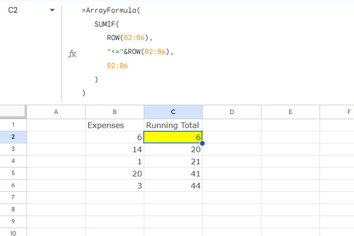
Clear the range C2:C6 and enter the following formula in C2:
=ArrayFormula(
   SUMIF(
      ROW(B2:B6),
      "<="&ROW(B2:B6),
      B2:B6
   )
)Note: We use ARRAYFORMULA because the ROW function is applied to a range.

Formula Breakdown:
The syntax follows: SUMIF(range, criterion, sum_range)
In the formula:
- range:
ROW(B2:B6)— This generates an array of row numbers corresponding to the rangeB2:B6(e.g., {2, 3, 4, 5, 6}). - criterion:
"<=" & ROW(B2:B6)— This creates a condition that checks if each row number in the range is less than or equal to the current row number. - sum_range:
B2:B6— This is the range of values that will be summed based on the specified condition.
For each row in B2:B6, the formula sums all the values in B2:B6 up to and including that row, resulting in a running total.
Additional Notes:
When using this running total array formula with an open range, ensure you include an IF logical test to return a blank when a value in the range is empty.
=ArrayFormula(IF(B2:B="", ,
   SUMIF(
      ROW(B2:B),
      "<="&ROW(B2:B),
      B2:B
   )
))
You can also replace the ROW function with a combination of SEQUENCE and ROWS:
=ArrayFormula(IF(B2:B="", ,
   SUMIF(
      SEQUENCE(ROWS(B2:B)),
      "<="&SEQUENCE(ROWS(B2:B)),
      B2:B
   )
))
This approach is particularly useful when the values for calculating the running total are generated from expressions (outputs of other functions such as QUERY, SORT, FILTER, etc.).
Other Array Formula Options for Running Total
Below are three options involving MMULT, DSUM, and SCAN. The first one is widely used in Excel. Running a total using DSUM is a unique idea and less popular, while SCAN is simpler but relies on the LAMBDA function. SCAN, like SUMIF, is also a popular option. Let’s explore each of them.
Using MMULT
We can use the following MMULT formula to calculate the running total in Google Sheets:
=ArrayFormula(
   MMULT(
      IF(ROW(B2:B6)>=TRANSPOSE(ROW(B2:B6))=TRUE, 1, 0),
      N(B2:B6)
   )
)
For a detailed explanation of the formula, please refer to my guide: Running Total Array Formula in Excel.
In Google Sheets, I’ve added the ARRAYFORMULA function along with MMULT.
However, in Excel, you can either enter the formula using Ctrl+Shift+Enter (legacy array method) or if using Office 365, it may spill the result automatically.
In Google Sheets, we can use open ranges starting from any row in formulas. If you want to use B2:B instead of a specific range like B2:B6, you can apply the formula below:
=ArrayFormula(IF(LEN(B2:B),
   MMULT(
      IF(ROW(B2:B)>=TRANSPOSE(ROW(B2:B))=TRUE, 1, 0),
      N(B2:B)
   ),
))
I don’t recommend using this for large datasets, and it’s included here for educational purposes only. The formula is resource-intensive because it uses MMULT with ROW and TRANSPOSE, creating a large matrix that grows quadratically with the number of rows.
Using DSUM
The DSUM function is another option for creating a running total array formula in Google Sheets. Since it’s a database function, we need to format the values in the range B2:B6 in a way that mimics a database structure.
The formula below returns the running total for the values in B2:B6:
=ArrayFormula(
   DSUM(
      TRANSPOSE(
         {B2:B6, IF(SEQUENCE(5, 5)^0 +
         SEQUENCE(1, 5, ROW(B2)-1)<=ROW(B2:B6),
         TRANSPOSE(B2:B6))}
      ),
      SEQUENCE(ROWS(B2:B6), 1), {IF(,,);
      IF(,,)}
   )
)
You can also modify this formula to work with an open range, such as B2:B. For a detailed explanation of how it works, check out the guide Running Max Values in Google Sheets, where a similar approach is explained.
Running Total with SCAN Function
The SCAN function is a newcomer to cumulative sum array formulas in Google Sheets. As a LAMBDA helper function (LHF), it provides a simple way to calculate a running total.
For a fixed range, the following formula works:
=SCAN(0, B2:B6, LAMBDA(a, v, (a+v)))The SCAN function processes the array B2:B6 and returns intermediate running totals.
In the formula:
0: The initial value (starting point) in the accumulator.B2:B6: The range to sum.LAMBDA(a, v, a + v): Adds each value (v) to the cumulative total (a), producing a running total at each step.
To apply this to an open range (e.g., B2:B), use the following:
=ArrayFormula(IF(B2:B="",,SCAN(0, B2:B, LAMBDA(a, v, (a+v)))))Resources
- Array Formula for Conditional Running Total in Google Sheets
- Reverse Running Total in Google Sheets (Array Formula)
- How to Calculate a Horizontal Running Total in Google Sheets
- Reset Running Total at Every Year Change in Google Sheets (SUMIF Based)
- Running Total by Category in Google Sheets (SUMIF Based)
- Running Total with Monthly Reset in Google Sheets (Array Formula)
- Custom Named Function for Running Total by Group (Item, Month, or Year)
- Weekly and Biweekly Running Totals in Google Sheets
- Reset Running Total at Blank Rows in Google Sheets
- Running Total with Multiple Subcategories in Google Sheets
- How to Add a Running Total in Pivot Table in Google Sheets


Hello, your running total array formula worked for me:
=ArrayFormula(If(len(B2:B),(SUMIF(ROW(B2:B),"<="&ROW(B2:B),B2:B)),))How can I amend this to check a date column and begin a new running total with each new year?
Hi, The Jay Jetson,
Have you checked the first tutorial under the related topic section below the post?
That’s a resource-hungry formula and may slow down your sheet in case you have a large set of data in it.
I have an alternative formula that involves a helper column. If you are interested, please let me know and share a sample sheet (leave the URL in your reply).
Hi, The Jay Jetson,
Please check my new tutorial here – Reset Running Total at Every Year Change in Google Sheets (SUMIF Based)
I have an improvement on SUMIF.
You don’t need to wrap it in an IF statement, if in the criterion you enter a SEQUENCE. Your example would look like this:
=ArrayFormula( SUMIF( ROW(B2:B), "<="& SEQUENCE(COUNT(B2:B),1,2), B2:B) )Hi, Giovanni Cipriani,
Imagine the range is B2:B10 and B5 is empty. Try your formula. It won’t work correctly.
Hello! Apologies if I’ve missed it, is there a way to add a bunch of video runtimes? For example, here is an excerpt of some runtime data in hours/minutes/seconds/milliseconds.
00:00:02:04
00:00:02:05
00:00:01:14
00:00:01:12
00:00:06:00
If I am to summarize the duration of all the videos added together, is there a formula for that? Thank you in advance.
Hi, Laura,
It seems the format is not correct. You may want to replace the last colon with a period.
Then you can sum it.
You can use Regex to Replace the Last Occurrence of a Character in Google Sheets.
If the above data is in B2:B6, you can try this formula.
=text(ArrayFormula(sum(value(REGEXREPLACE(B2:B6,"(.*)\:","$1.")))),"hh:mm:ss.000")Hi there! I would like to implement an auto-expanding running balance, but add one criterion. The problem is that SUMIF doesn’t allow me to do that, and SUMIFS doesn’t auto-expand. Is there a good solution?
Hi, Jeffrey,
As you have mentioned, I also think SUMIF or SUMIFS won’t work. But I do have an array formula. Please stay tuned for my update below!
Hi, Jeffrey,
I hope this conditional running sum array formula would give you some idea.
https://infoinspired.com/google-docs/spreadsheet/conditional-running-total-array-formula-google-sheets/
Thanks, Prashanth! For some reason, I wasn’t notified of your response by email, but I noticed the new article from your Twitter account 🙂
When I placed this formula into my Gsheet, it puts a 0 in the first row of the total column instead of the total for the first row and it displays the total for the first row on the 2nd row. So all of my totals are 1 row lower than they should be.
Any idea how to fix this?
Hi, Chris,
No idea! You can check my example Sheet included in the post.
Best,
Hi,
The one-line array formula worked perfectly for me. Thanks for saving me a ton of time.
In formula #2, the word “obsolete” should be “absolute”. The dollar sign makes it an absolute address instead of a relative address.
Hi, Michael,
Thanks for pointing out the error.
Corrected that and also included few links related to running count calculation in Sheets.
Best,