Preparing an amortization schedule in Google Sheets is pretty easy with the built-in PMT, PPMT, and IPMT functions. But when you want to include extra principal payments in your schedule, you may want to follow a different approach.
This tutorial covers the following two topics in detail.
- How to create an amortization schedule in Google Sheets.
- Amortization schedule with extra principal payments in Google Sheets.
Please note that the below two amortization schedules are based on constant amount periodic payments and that at a constant interest rate.
Amortization Schedule Calculation in Google Sheets Using the Built-in Functions
We can use some of the financial functions in Google Sheets to create a loan amortization schedule easily. No matter your periodic payments are on a weekly, fortnightly, quarterly, or monthly basis, the same formulas would help.
First I will explain to you how to create an amortization schedule in Google Sheets that involves monthly (periodic) payments.
Here are the steps to create an amortization schedule/table in Google Sheets.
We need the following input values.
- Loan Amount.
- Annual Interest Rate of the Loan.
- Duration in Years.
Step 1: Input Values in Amortization Schedule.
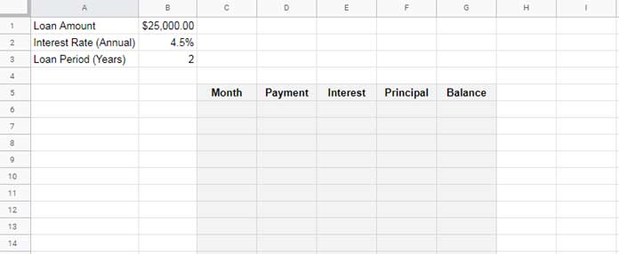
Please arrange the values as per the below image.

Step 2: Preparing Amortization Table Format.
We need a 5 column table to enter the formulas. You can create that format as below.
The Formulas to Create an Amortization Schedule in Google Sheets
In my example, the loan period is set to 2 years in cell B3. That means there are 24 periodic payments.
Number of Payments in Sequential:
In cell C6, enter the below ROW formula to get the number of periods in sequential order.
=ArrayFormula(row(1:24))Payment Calculation (Monthly Payments Including Interest + Principal Payment):
In cell D6, we can use the below PMT formula to calculate the monthly payments.
=-pmt($B$2/12,$B$3*12,$B$1)You need to drag this formula down until the cell D29. So as an alternative I am converting the above PMT formula as an array formula.
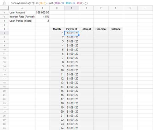
Since the payment is the same for each period (constant periodic payments) I have used an array formula to fill all the 24 periods with the PMT value.
Just enter this PMT formula in cell D6 and let it auto expand to cell D29!
=ArrayFormula(if(len(C6:C),-pmt($B$2/12,$B$3*12,$B$1),))It will look like as below.
Interest Calculation Using IPMT:
You can use the below IPMT formula in cell E6 and drag down until it reach the cell E29.
=-ipmt($B$2/12,C6,$B$3*12,$B$1)You can also convert the above IMPT formula to an expanding array formula. Here is that.
=ArrayFormula(if(len(C6:C),-ipmt($B$2/12,C6:C29,$B$3*12,$B$1),))I am including the non-array formula to make you understand the formula better. You can use the array formulas only.
Principal Payment Calculation Using PPMT:
Enter the below PPMT formula in cell F6:
=-ppmt($B$2/12,C6,$B$3*12,$B$1)This is equal to Payment – Interest. So instead of PPMT, the below basic formula would also return the correct result.
=D6-E6You can use any of the above formulas in cell F6 and drag/copy down. Here is the array version of the PPMT formula.
=ArrayFormula(if(len(C6:C),-ppmt($B$2/12,C6:C29,$B$3*12,$B$1),))Remaining Balance Amount:
In cell G6 enter the below formula and drag down.
=$B$1-sum($F$6:F6)Follow the above steps to prepare an amortization schedule in Google Sheets.
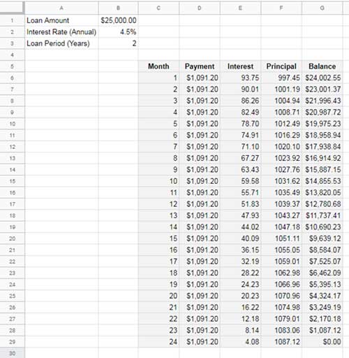
Finished Table:
Tips to Change Amortization Schedule Payment to Weekly, Fortnightly, or Quarterly Basis
Many people think it’s tough to change the monthly periodic payment in financial functions. It’s not so.
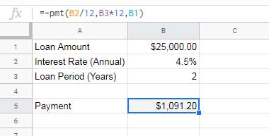
Here in cell B2 we have the annual interest rate. Let me explain how to change that based on your periodic payments.
Weekly Interest Rate = Yearly Interest Rate / 52
Fortnightly Interest Rate = Yearly Interest Rate / 26
Monthly Interest Rate = Yearly Interest Rate / 12 (this what I have used in the formula in cell B5)
Quarterly Interest Rate = Yearly Interest Rate / 4
In cell B3 we have the loan period in years. So multiply it with 52, 26, 12 or 4 based on your periodic payments.
So in my all formulas (above and below) you can change interest /12 to interest/? and the number of periods * 12 to number of periods * ?.
Note: Replace the question mark with the periodic payment (52, 26, 12, and 4) that you want.
Creating an Amortization Schedule With Extra Principal Payments in Google Sheets
In case you want to make extra payments, the Google Sheets built-in functions except the PMT won’t help. We have to follow a different approach here. That also not much complicated.
Here also I am following the same above input values and format. But this time you must include a new column to show your extra principal payments in each period.

Here in this amortization schedule the Payment (column C) amount will be the same. I mean in comparison with the above amortization schedule that doesn’t include any extra principal payments.
If the Extra Principal payment column is blank (column F), then the Interest payment (column D), as well as the Principal payment (column E), will also be the same (compared to the earlier schedule).
That means we can use the PMT function to calculate the Payment (column C). To calculate the Principal payment (column E) and Interest payment (column D), we can use custom formulas.
Before proceeding to the tutorial please see the input values again in the above screenshot.
Formulas Involved in Amortization Schedule With Extra Principal Payments
Sequential Numbers in the Range B10:B26:
Enter the number 1 to 17 in the said range. I am not using the ROW formula this time.
Actually there are 24 months (2 years) and the payment is monthly. Then why I am using 17 months?
I am going to make $500.00 as extra principal payments every month. So the future value (FV) will be 0 at the completion of the 17th month.
PMT Formula to Calculate the Periodic Payment in Cell B5:
This time I am using the PMT formula in cell B5, not in cell C10. In cell C10 we will get the same value but there we must include a logical IF statement.
First enter this formula in cell B5.
=-pmt(B2/12,B3*12,B1)Also in cell G9 get the Loan Amount. You can use this formula in cell G9.
=B1Now your sheet must look like as below.
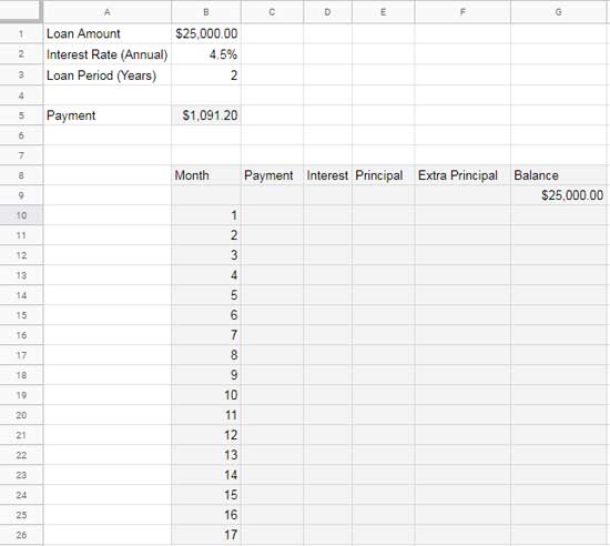
Amortization Schedule With Extra Principal Payments – Custom Formulas
PMT with IF Logical:
In cell C10, use this formula to get the PMT value that available in cell B5.
=IF($B$5<=G9,$B$5,G9+(G9*$B$2/12))This formula checks the balance column G in the immediate row above. For example, the formula in cell C10 checks the value in cell G9.
If the value in cell B5 (PMT) is less than the value in cell G9, the formula would return the value in cell B5 as it is. That means the PMT value will retain.
Once the value in cell B5 (PMT) becomes greater than the balance value in column G, the logical test executes the highlighted part (see image below). That is;
PMT = Balance Payment (G25) + Monthly Interest (G25*$B$2/12)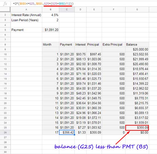
Manual IPMT with IF Logical:
You can calculate the interest payment using custom formula as below.
IPMT = Balance Payment (G9) x Monthly Rate ($B$2/12)So enter this formula in cell D10 and drag down. I have used the IF logical here to check the presence of PMT in column C.
=IF(len(C10),G9*$B$2/12,0)Manual PPMT with IF Logical:
Since you have already the PMT (periodic payment) and interest (IPMT) in hand, you can easily calculate the principal payment amount.
Principal Payment (PPMT) = Payment Amount (PMT) - Interest Payment (IPMT)So the formula to use in cell E10 is;
=IF(len(C10),MIN(C10-D10,G9),0)Of course, you must copy this formula down. Then fill the column F with the extra principal payments, i.e. $500.00 in the range F10:F25.
Finally, in cell G10 enter the below formula to calculate the balance which must also be dragged down.
=IF(G9>0,G9-E10-F10,0)That’s all. If you have any doubt, please check my example Sheet.


