By now, you may have tried different formula variations to aggregate text strings using the QUERY function in Google Sheets. No success, right?

You’re not alone. Many users wonder how to use aggregate functions in QUERY for strings—it’s a topic often discussed online.

It’s commonly believed that Google Sheets QUERY doesn’t support text string aggregation, and that’s only partially true.

Why Only Partially?

Because you can use the aggregation functions MIN or MAX in the QUERY SELECT clause with strings! These functions can help achieve our goal.

Note: It’s not possible to use CONCATENATE or other text join functions directly within QUERY.

Aggregate Strings in Google Sheets with QUERY: What Does It Mean?

Let’s clarify this concept with an example.

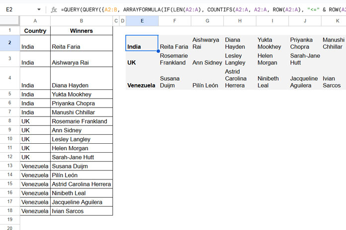
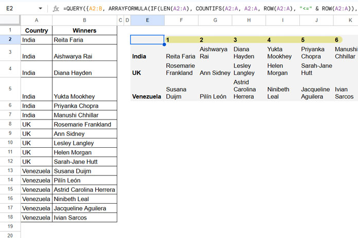
My sample data is in columns A and B, where A contains country names, and B contains Miss World Pageant winners. The dataset includes three countries for simplicity and clarity.

Using QUERY, the data in column A (countries) can be grouped, and the corresponding values in column B (winners) can be aggregated.

To achieve this, we’ll use a helper column. If you’re not keen on adding a helper column, we’ll also explore an alternative with a virtual helper column.

Example: Aggregate Strings Using QUERY in Google Sheets

Helper Column Approach:

We’ll use the sample dataset mentioned earlier.

Step 1:

Since this is a helper column approach, enter the following formula in cell C2 (the helper column):

=ARRAYFORMULA(IF(LEN(A2:A), COUNTIFS(A2:A, A2:A, ROW(A2:A), "<=" & ROW(A2:A)),))

This formula generates a sequential count for each group of data in column A. For a detailed explanation of this formula, refer to my tutorial: Running Count in Google Sheets: Formula Examples.

Step 2:

Use the following QUERY formula in cell E2 to aggregate the text strings:

Formula 1:

=QUERY(QUERY(A2:C, "Select Col1, max(Col2) where Col1 is not null group by Col1 Pivot Col3"), "Select * offset 1", 0)

This formula aggregates the strings, and the result will match the image above.

Without Using a Helper Column:

If you prefer not to use a helper column, you can use the formula below directly in cell E2, skipping Step 1:

Formula 2:

=QUERY(QUERY({A2:B, ARRAYFORMULA(IF(LEN(A2:A), COUNTIFS(A2:A, A2:A, ROW(A2:A), "<=" & ROW(A2:A)),))}, "Select Col1, max(Col2) where Col1 is not null group by Col1 Pivot Col3"), "Select * offset 1", 0)

Here, the helper column formula from Step 1 is integrated into the QUERY as a virtual column.

Both formulas work seamlessly with sorted or unsorted group column data. However, sorted data has one advantage: the first column of the aggregated data will naturally be in sorted order. The aggregated strings, however, will not be sorted.

If you want the aggregated strings to also be in sorted order, sort the source data first. To do this, select the range A1:B, then click Data > Sort range > Advanced range sorting options. Check the box for “Data has a header row,” select “Sort by Country” in ascending order, and click “Add another sort column.” Choose “Winners” and sort it in ascending order as well.

Formula Explanation

Inner QUERY:

The inner QUERY aggregates the strings.

• QUERY(A2:C, "Select Col1, max(Col2) where Col1 is not null group by Col1 Pivot Col3")
  • Select Col1, max(Col2): Groups the data by Col1 (Country) and computes the maximum value of Col2 (Winners) for each group.
  • Pivot Col3: Distributes the results across columns based on the values in Col3 (Helper column). This ensures the “max” winner for each running count is arranged in its corresponding position.

The result of this QUERY is a table where:

• Each row corresponds to a unique value in Col1 (Country).
• Columns correspond to Col3 (Helper values), showing the “max” winners for each sequence.

Outer QUERY:

The outer QUERY cleans up the aggregated strings by removing the header (Helper Column Values).

• QUERY(..., "Select * offset 1", 0)
  • Select *: Retains all columns from the inner QUERY result.
  • Offset 1: Skips the first row (header row generated by the pivot).

This is how the formula Aggregate Strings in Google Sheets Using QUERY.

Resources

• VLOOKUP and Combine Values in Google Sheets
• How to Use VLOOKUP on Duplicates in Google Sheets
• How to Unstack Data into Groups in Google Sheets
• Unstack Multiple Form Responses in Google Sheets
• How to Stack Data in Google Sheets: Tips and Tricks
• A Simple Formula to Unpivot a Dataset in Google Sheets
• EXPAND + Stacking: Expand an Array in Excel
• Unpivot Excel Data Fast: Power Query & Dynamic Array Formula