In-cell progress bars in Excel refer to bars that are within a cell, not floating above it. They can be aligned vertically or horizontally within the cell.

We will utilize conditional formatting for the horizontal progress bar, whereas, for the vertical progress bar, we will utilize the sparklines column chart.

Both methods will dynamically adjust the size of the progress bar within the cell based on changes in the percentage value.

Horizontal Progress Bar Using Conditional Formatting in Excel

Here are the step-by-step instructions:

Cell B3 contains the value 75%, representing the percentage completion of a task.

Conditional Formatting:

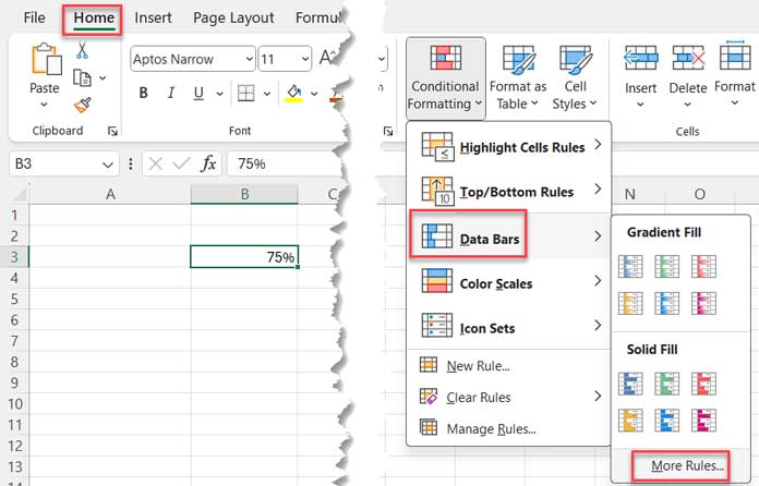
1. Navigate to cell B3.
2. Go to the Home tab and select Conditional Formatting > Data Bars > More Rules.
   
3. This will open the New Formatting Rule dialog box as follows.
   
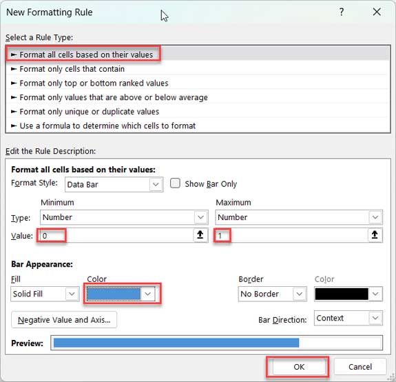
4. Make sure the selected rule type is “Format all cells based on their values.” If not, select it.
5. Under “Minimum,” select “Number” and enter 0 (representing 0%).
6. Under “Maximum,” select “Number” and enter 1 (representing 100%).
7. Select a fill color; for example, we’ll choose “Dark Blue.” Choose the color you prefer.
8. Click OK.

This will create a horizontal progress bar in cell B3.

Other Customizations:

Adjust the column width and row height as per your requirements.

Additionally, you can align the percentage value within the cell to the left, center, or right horizontally, and to the top, middle, or bottom vertically. You can also adjust the font size and color. These options are available in the Font and Alignment groups under the Home tab.

When you update the value in cell B3, the changes will be reflected in the horizontal progress bar. You can use the format painter to apply this conditional formatting to other cells.

Vertical Progress Bar Using Sparklines in Excel

To create an in-cell vertical progress bar, we will use the Sparklines chart in Excel. Here are the step-by-step instructions:

The value in cell B3 is 75% for the test.

1. Navigate to cell B3.
2. Go to the Insert tab and click on Column within the Sparklines group.
3. In the dialog box that opens, select cell B3 under “Choose where you want the sparklines to be placed.”
   
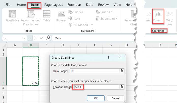
4. Click OK.
5. If the active cell is B3, you will see a new tab named “Sparklines.” Go to that tab and click “Axis,” then select “Custom value” under the “Vertical Axis Minimum Value Options” and overwrite the existing value with 0 (representing 0%).
6. Again click “Axis” and select “Custom value” under “Vertical Axis Maximum Value Options” and overwrite the existing value with 1 (representing 100%).
   
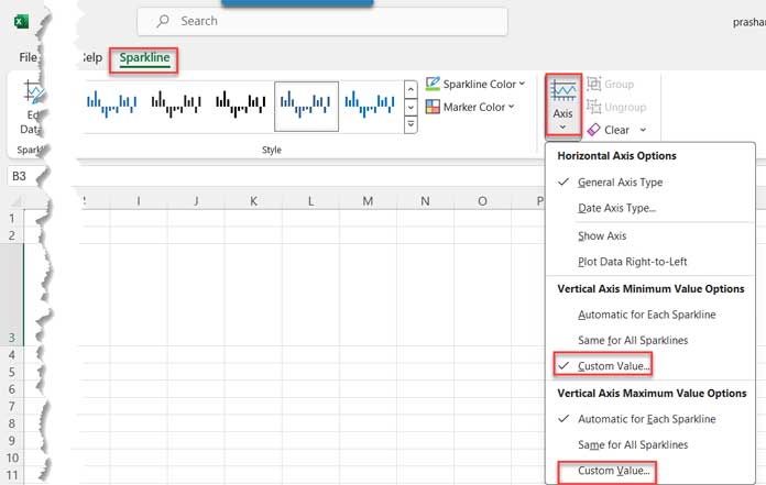
7. Select the color of the vertical progress bar by clicking “Sparkline Color” in the “Style” group under the Sparkline tab. You can find this option next to the “Axis” settings. Please refer to the screenshot above for clarity.

This will create an in-cell vertical progress bar in Excel.

Percentage Value Customization:

Here are some optional customizations to enhance the visual appeal of the progress bar.

Increase the row height and column width as desired. Similar to the horizontal progress bar, you can align the percentage value to the left, center, or right horizontally, and to the top, middle, or bottom vertically from the Home tab. Additionally, you can adjust the font size and color.

When you update the value in cell B3, the changes will be reflected in the vertical progress bar.

To create additional bars, simply copy and paste the sparkline into another cell and modify the percentage value in the cell.

Conclusion

In addition to the above, for in-cell horizontal progress bars, you can use the TEXT function in Excel. This involves repeating a character based on the percentage value. However, it’s worth noting that this method may not be 100% accurate.

Therefore, in Excel, conditional formatting and Sparklines remain the best two options for creating in-line progress bars.