


This post explains how to use OR criteria in COUNTIFS in either of the columns in Google Sheets.
The best way to solve this is using QUERY. But if you wish to use COUNTIFS, you may want to use it not in the usual way.
I will share both formulas here. Before that, here is the scenario to understand the problem.
Assume five teams compete with each other in a tournament.
So there are two columns (C and D) in a spreadsheet with the following data.
Team (column C) Vs Team (Column D):
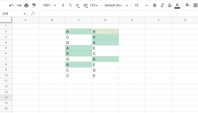
I want to see how many matches have been played by teams A or B so far.
In other words, whether the text/string A or B matches in either of the columns in each row.
As per the above example, there are corresponding data in 7 rows.
One match A & B plaid against each other and six matches with the other teams.
So the output must be 7, not 8.
To get this, we must know how to use OR criteria in COUNTIFS in either of the columns.
You May Like:- How to Use All Google Sheets Count Functions [All 8 Count Functions].
How to Use OR in COUNTIFS in Either of the Columns in Google Sheets
For counting based on more than one condition, the dedicated function is COUNTIFS.
How to use it for our purpose here?
I’ve earlier posted two related tutorials.
- COUNTIFS with Multiple Criteria in the Same Range in Google Sheets.
- OR in Multiple Columns in COUNTIFS in Google Sheets.
They are slightly different from our new problem, i.e., OR in COUNTIFS in either of the columns.
Formula_1:
=ArrayFormula(SUM(COUNTIFS(if((C2:C="A")+(C2:C="B"),"~","")&if((D2:D="A")+(D2:D="B"),"~",""),{"~","~~"})))The above is the solution to OR in COUNTIFS in either of the columns in Google Sheets.
How Does This Formula Work?
If you check either of the above tutorials, preferably the first one, you can understand the basics.
There I have used a virtual array formed using Curly Braces to use OR in one column.
Here is a quick example.
We can use the following formula to count the fruits “dragon fruit” or “papaya” in column A.
Generic Formula for OR in COUNTIFS in Either of the Columns: =ArrayFormula(SUM(COUNTIFS(criteria_range,{criterion_1,criterion_2,...})))
=ArrayFormula(SUM(COUNTIFS(A:A,{"dragon fruit","papaya"})))criteria_range – A:A
criterion_1 – “dragon fruit”
criterion_2 – “papaya”
We have followed this in formula_1 above after virtually modifying the source data.
I’ll explain the steps with the help of a few helper columns.
Insert the following formula in cell F2.
=ArrayFormula(if((C2:C="A")+(C2:C="B"),"~",""))It matches the teams’ A or B in column C and returns a tilde mark in matching rows.
Insert the below formula in cell G2 to match teams A or B in column D and return a tilde.
=ArrayFormula(if((D2:D="A")+(D2:D="B"),"~",""))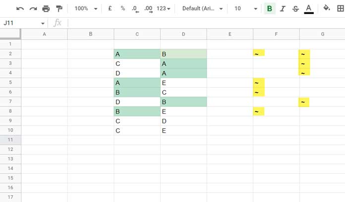
Related: How to Use IF, AND, OR in Array in Google Sheets.
When you combine both, we will get our criteria_range.
=ArrayFormula(if((C2:C="A")+(C2:C="B"),"~","")&if((D2:D="A")+(D2:D="B"),"~",""))So the criteria will be as follows.
criterion_1 – “~”
criterion_2 – “~~”
I hope it goes without saying.
OR in COUNTIFS in Either of the Columns – Alternative Formula Using Query
We cause a QUERY alternative in Google Sheets to solve the OR in COUNTIFS in either of the columns’ problems.
Here is that formula.
=query(C2:D,"select count(C) where C matches 'A|B' or D matches 'A|B' label Count(C)''")As you can see, to get the count as per our requirement, I have used the Matches regular expression match, one of the complex comparison operators, in the Where clause.
That’s all. Thanks for the stay. Enjoy!
Resources
- COUNTIFS in a Time Range in Google Sheets [Date and Time Column].
- Varying Array Sizes in COUNTIFS in Google Sheets.
- Google Sheets: COUNTIFS with Not Equal to in Infinite Ranges.
- Countif | COUNTIFS Excluding Hidden Rows in Google Sheets.
- How To Use Countif or COUNTIFS In Merged Cells In Google Sheets.
- Not Blank as a Condition in COUNTIFS in Google Sheets.