How to copy-paste merged cells’ values without blank rows in Google Sheets?

Without copy-paste commands, transferring data thru’ a computer’s interface won’t be easier as we think. On Windows, you can use Ctrl+C to copy and Ctrl+V to paste. On Mac, just use the ‘Command’ key instead of the Ctrl.

In Google Sheets, we can use these commands to complete our tasks ASAP. I am not undermining the importance of the Cut command. It’s equally useful.

Other than the above commands there is a special command in Google Sheets and it’s ‘Paste special. I’ll come back to this.

There is no option in Google Sheets to copy-paste merged cells without blank rows or spaces. If you copy and simply paste, the values will be pasted as it is.

If you apply the paste special (Ctrl+Shift+V), then the values will be pasted as un-merged but with blank cells. Then what about pasting the copied values to another application? Se the below screenshots.

• Extra blank rows in the pasted (paste special) column (column B) in Google Sheets (Screenshot # 1).

• Extra spaces in Notepad (Screenshot # 2).

To copy-paste merged cells without blank rows as well as spaces, you can follow the below approaches.

How to Copy and Paste Merged Cells Without Blank Rows in Sheets

If your purpose is to just copy the merged cells’ values in a column to another column that without blank rows in between, use the Filter formula.

For example, consider the scenario # 1 (screenshot # 1) above. In that in column B that ideally, in cell B1, you can use the below Filter formula.

=filter(A1:A,A1:A<>"")

It will filter out blank rows. In other words, it will extract the values in column A leaving blank rows caused by merging of rows.

Query is another way to remove blank rows from a merged column of data.

=query(A1:A,"Select A where A<>''")

What about scenario # 2? I mean how to paste the above values in column A to notepad without spaces. No more extra steps here. Use the Filter/Query formula and copy that formula output to Notepad.

Merged Cells to Unmerged Cells – Multiple Columns

In the case of merged cells in multiple columns, you can use the above Query formula as below.

Example: Merged cells in column A and B and the Query output in column D.

=query({A1:A;B1:B},"Select Col1 where Col1<>''")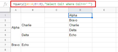

Here as you can see the formula returns the values in merged cells in two columns into a single column. If you want the output in two columns, you can use the earlier filter formula in cell D1 and drag to the right.

See that the values in each columns are getting pasted to adjacent cells to the down and right.

That’s all about how to copy-paste merged cells without blank rows in Google Docs Sheets. Thanks for the stay, enjoy!

More Google Sheets Tips and Tricks:

1. How to Count If Not Blank in Google Sheets [Tips and Tricks].
2. Vlookup in Google Sheets – 10 Formula Variations, Tips, and Tricks.
3. 10 Best Tick Box Tips and Tricks in Google Sheets.
4. How to Fill 0 in Blank Cells in Google Sheets [Tips and Tricks].
5. Date Related Conditional Formatting Rules in Google Sheets.