How do I match two columns that contain values not in any order in Google Sheets? I can suggest to you four different formulas using four different functions.
The functions include Vlookup, Countif, Query, and Regexmatch. Here I am going to use the Regexmatch function to match two columns that contain values not in any order in Google Sheets.
What about the other three functions. All that has already been covered and see that links.
1. Match two columns using the Vlookup function.
2. The Countif based formula to match columns.
3. The Query formula to compare and remove duplicates.
Here in this Google Sheets tutorial, I am going to detail you how to do it with the REGEXMATCH function.
Values in Order:
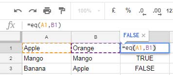
To compare two columns that in an order you can use the EQ Operator function or the equivalent ‘==’ operator. Everybody knows this.
In this comparison, the values should be from the same row but from two different columns.

Values Not in Order:
When you want to compare two columns and the values in that columns are not in any order, you can use any of the three formulas that I’ve mentioned above. Here is the fourth one that using Regexmatch.

If the column values are numeric, additionally you should use the To_Text function otherwise the Regex won’t work. Let me explain all these.
How to Match Two Columns that Contain Values Not in Any Order Using Regex in Google Sheets?
Regexmatch Formula to Compare Two Text Columns
=ArrayFormula(regexmatch(A1:A3, textjoin("|", 1, B1:B3)))
This formula is for the above range. If you want this formula to automatically adjust to the last nonblank row, use the IF and LEN combo as below with the formula above.
=ArrayFormula(if(Len(A1:A),regexmatch(A1:A, textjoin("|", 1, B1:B)),))
As you can see, the above formula uses the RE2 regular expressions to compare two columns that are not in any particular order.
How does this Regexmatch formula compare Columns?
Maybe you are interested to see the Regexmatch Syntext.
REGEXMATCH(text, regular_expression)
In this, the argument text is the values in Column A1: A. The regular expression is the Textjoin formula that joins the column B1: B values as below.

The formula works like this. Just leave the above example aside.
Suppose I want to check the presence of either of the two strings (Japan or China) in A1. Here is the suitable Regexmatch formula.
=REGEXMATCH(A1, "Japan|China")
Now take a look at Cell E1 in the above image. I’ve combined the values in Colum B to use it as the regular expression in Query. Hope you could understand the Regexmatch logic above.
Regexmatch Formula to Compare Two Numeric Columns
You should feed text values to Regex as it’s text function. If you want to use Regex in columns containing numeric, date or time values, you should use the To_Text function to convert the numeric values to text values.
=ArrayFormula(if(Len(A1:A),regexmatch(to_text(A1:A), textjoin("|", 1, to_text(B1:B))),))
Just wrap the range with the To_text function to convert the numeric values to text. This way you can use Regexmatch with numeric columns.
Use Regex and match two columns in Google Sheets. Enjoy!


