XLOOKUP Nth Match in Google Sheets – How to Return the Nth Occurrence

Sometimes, you may need to retrieve the Nth occurrence of a value from a dataset using XLOOKUP in Google Sheets. This is especially useful when you have repeated entries and want to extract a specific match, not just the first one.

Let’s explore how to perform XLOOKUP Nth Match in Google Sheets with a real-world example.

Sample Data

In this tutorial, we’ll be working with sample data that consists of three columns:

Month (Column A) – the month in which the data was recorded.
Country (Column B) – the country where the data was collected.
No. of Employees Engaged (Column C) – the number of employees engaged in that month and country.

For example:

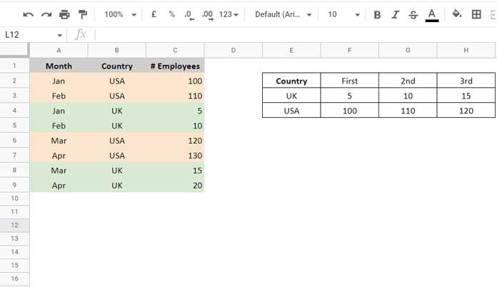
Sample data for XLOOKUP Nth Occurrence in Google Sheets

The purpose of this tutorial is to show you how to use XLOOKUP Nth Occurrence to find the Nth match (e.g., the second or third instance) of a country and return the corresponding value from another column, such as No. of Employees Engaged.

By the end of this guide, you’ll be able to quickly locate specific data points, even when multiple matches exist.

Why Not Just Use FILTER + INDEX?

Yes, you can use a combination like:

=INDEX(FILTER(C2:C10, B2:B10="USA"), 3)

This returns the third occurrence of USA from column C.

However, this method lacks XLOOKUP‘s features like:

wildcard matching,
directional search (first-to-last or last-to-first),
and compatibility with structured arrays.

Let’s instead use XLOOKUP Nth Occurrence in Google Sheets to unlock more flexibility.

1. XLOOKUP Nth Match in Google Sheets (Search First to Last)

Assume we want to get the Nth value of “USA” or “UK” from the Country column and return the matching value from No. of Employees Engaged.

We’ll place our search terms in E3:E4:

E3: USA
E4: UK

1st Occurrence Formula (F3):

=ARRAYFORMULA(XLOOKUP(E3:E4, B2:B10, C2:C10, "", 0, 1))

This will return 100 for USA and 5 for UK.

2nd Occurrence Formula (G3):

=ARRAYFORMULA(
  LET(
    rc, COUNTIFS(B2:B10, B2:B10, ROW(B2:B10), "<="&ROW(B2:B10)),
    n, 2,
    XLOOKUP(E3:E4, FILTER(B2:B10, rc=n), FILTER(C2:C10, rc=n), "", 0, 1)
  )
)

This returns:

110 for USA
10 for UK

3rd Occurrence Formula (H3):

Change n from 2 to 3:

=ARRAYFORMULA(
  LET(
    rc, COUNTIFS(B2:B10, B2:B10, ROW(B2:B10), "<="&ROW(B2:B10)),
    n, 3,
    XLOOKUP(E3:E4, FILTER(B2:B10, rc=n), FILTER(C2:C10, rc=n), "", 0, 1)
  )
)

This returns:

120 for USA
15 for UK

2. XLOOKUP Nth Occurrence in Google Sheets (Search Last to First)

To reverse the direction (bottom to top), update the running count logic.

Use:

=ARRAYFORMULA(
  LET(
    rc, COUNTIFS(B2:B10, B2:B10, ROW(B2:B10), ">="&ROW(B2:B10)),
    n, 2,
    XLOOKUP(E3:E4, FILTER(B2:B10, rc=n), FILTER(C2:C10, rc=n), "", 0, -1)
  )
)

This will search from last to first and return:

120 for USA (Mar)
15 for UK (Mar)

Change n to target different occurrences from the bottom.

Note: Replacing 1 with -1 in the search_mode is not strictly required here because we’re using filtered data. Whether you search from first to last or last to first, the result will be the same in this context.

3. XLOOKUP with Wildcards for Nth Match

Let’s say you want to match “US” with both “USA” and possibly “US-East” (if data expands). Use wildcards in XLOOKUP Nth Occurrence in Google Sheets by updating the match mode and appending *.

Example formula:

=ARRAYFORMULA(XLOOKUP(E3:E4&"*", B2:B10, C2:C10, "", 2, 1))

Set E3:E4 to:

E3: US
E4: UK

This will match values like “USA”, “US-East”, and return their respective employee counts.

Note: This wildcard approach is applicable to all the XLOOKUP Nth Match formulas above — whether you’re searching from top to bottom, bottom to top, or matching the Nth occurrence.

Summary

Use COUNTIFS with LET and FILTER to isolate the Nth match.
Control direction using search_mode: 1 = first to last, -1 = last to first.
Use wildcards (*) with match_mode = 2 for partial matches.

With this guide, you’re now equipped to use XLOOKUP Nth Match in Google Sheets effectively — even with multiple conditions or reverse search.