Do you know the purpose of the ARRAY_CONSTRAIN formula in Google Sheets? Perhaps not, as this function is not as widely known, and there are alternative functions available.

The ARRAY_CONSTRAIN function proves to be quite useful on specific occasions. It’s important not to confuse this function with Google Sheets ARRAYFORMULA, as they serve different purposes, with the latter being more powerful.

Let me explain the use of the ARRAY_CONSTRAIN Formula in Google Sheets.

The main purpose of the ARRAY_CONSTRAIN function is to limit the result of an array to a specified number of rows and columns. This allows us to restrict both the number of rows and columns in the output.

In other words, we can exclude a specific number of rows from the end of the array/range and also a specific number of columns from the end of the array/range.

If you need to shift (offset) or manipulate rows and columns, alternative functions like OFFSET, QUERY, or INDEX may be more suitable.

ARRAY_CONSTRAIN Function Syntax in Google Sheets

Syntax:

ARRAY_CONSTRAIN(INPUT_RANGE, NUM_ROWS, NUM_COLS)

Arguments:

input_range: The range to constrain, for example, A1:C20 or ‘sourcemaster’ (named range).

num_rows: The number of rows that the formula output should contain. For instance, in the above input_range A1:C20, there are twenty rows. You can limit those rows to 10 (A1:C10) in the result by specifying num_rows as 10.

num_cols: The number of columns the formula output should contain. In the above input_range, the number of columns is three. Limit that to 2 (A1:B20) by specifying num_cols as 2.

Basic Example: Constraining Rows and Columns

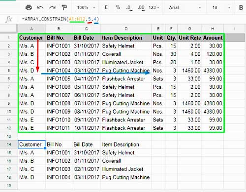
See the image below, which displays an ARRAY_CONSTRAIN formula in Google Sheets and its result. I’ve also marked all the parameters used in the formula for your quick reference.

Formula used in Cell A14:

=ARRAY_CONSTRAIN(A1:H12, 5, 4)

In this formula, A1:H12 represents the entire data range, also known as input_range. The formula is set to return 5 rows and 4 columns. Consequently, the result comprises the first 5 rows and the first 4 columns.

I applied the above formula in Cell A14, as illustrated in the image.

This example should provide clarity on the utilization of the ARRAY_CONSTRAIN function in Google Sheets.

Learn the Usage of the ARRAY_CONSTRAIN Formula with Practical Examples

Below, you can find two examples demonstrating the practical use of the ARRAY_CONSTRAIN function in Google Sheets.

These examples involve two popular functions – QUERY and FILTER. Even if you are not yet familiar with these functions, you can still follow the examples. Simply focus on the ARRAY_CONSTRAIN part.

ARRAY_CONSTRAIN Function in Conjunction with QUERY

Normally, there is no need to use the ARRAY_CONSTRAIN function with the QUERY formula, as you can limit the columns using the SELECT clause and rows using the LIMIT and OFFSET clauses within the QUERY function itself.

Must Read: What is the Correct Clause Order in Google Sheets Query?

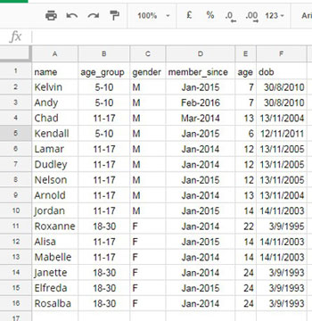
Consider the following QUERY formula, which retrieves rows containing the age_group ‘5-10’ in column B:

=QUERY(sourcemaster, "select A, B, C, D, E, F where B='5-10' limit 1", 1)

Note: ‘sourcemaster’ is a named range containing multiple rows and columns (A1:Z). The result will consist of 6 columns and two rows, including the header row.

In the QUERY LIMIT clause, you can specify the number of rows to return. However, for columns, you must individually specify them in the SELECT clause (e.g., select A, B, C, D, E, F), unless you are an advanced QUERY user.

For advanced QUERY users, there’s an option to automate column selection using the method explained in “How to Get Dynamic Column Reference in Google Sheets Query.”

Now, let’s explore how to use the Google Sheets ARRAY_CONSTRAIN function with QUERY to limit the columns. The following formula returns only two rows and six columns:

=ARRAY_CONSTRAIN(QUERY(sourcemaster, "select * where B='5-10' "), 2, 6)

In the QUERY, I used the asterisk (*) in the SELECT clause to output all columns in the ‘sourcemaster’ range. Then, I limited the output to 6 columns and 2 rows using ARRAY_CONSTRAIN.

This type of ARRAY_CONSTRAIN usage is beneficial when you need to return a large number of columns that are not easily specified one by one in the QUERY SELECT clause. Similarly, you can control the filter output to a specific number of rows.

ARRAY_CONSTRAIN Function in Conjunction with the FILTER Function

Here is another application of this function. First, observe this standard Filter formula:

=FILTER(MasterFile!A2:F16, MasterFile!B2:B16="5-10")

Below, I have constrained the output of the Filter formula with ARRAY_CONSTRAIN:

=ARRAY_CONSTRAIN(FILTER(MasterFile!A2:F16, MasterFile!B2:B16="5-10"), 2, 6)

Dynamic NUM_ROWS and NUM_COLS Parameters

In all the above examples, we have used predefined numbers such as 2 and 6 for num_rows and num_cols in the ARRAY_CONSTRAIN formulas.

Let’s explore how to use them dynamically, in other words, employ expressions for num_rows and num_cols.

Consider a sheet named “Sheet1” containing 1000 rows and 26 columns, i.e., A1:Z1000.

The first row contains headers, and the corresponding data is below in each column. We don’t know the total number of columns and rows that data fills.

If there are no blank cells in the header row A1:Z1 and the first column A1:A1000, you can use the following ARRAY_CONSTRAIN formula in another sheet in that file to filter only the data, excluding blank rows and columns.

=ARRAY_CONSTRAIN(Sheet1!A1:Z, COUNTA(Sheet1!A1:A), COUNTA(Sheet1!A1:Z1))

If “Sheet1” is empty, this formula will return a #REF! error, and you can’t eliminate it using IFERROR. In such cases, use conditional formatting, as explained in this tutorial: How to Remove #REF! Errors in Google Sheets (Even When IFERROR Fails).

Conclusion

The ARRAY_CONSTRAIN function in Google Sheets can be used in conjunction with other functions that return an array result.

Another function worth noting, which wasn’t initially mentioned, is SORTN in Google Sheets. SORTN can assist in limiting the number of rows in the output, though it will also sort the result.

Related Reading:

1. Three Different Ways to Limit Number of Rows in Google Sheets Query.
2. How to Offset Match Using Query in Google Sheets.