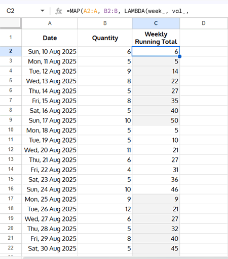
When working with data in Google Sheets, it’s often useful to calculate running totals to see how values build up over time. In this guide, I’ll show you how to set up weekly and biweekly running totals in Google Sheets using array formulas.
The difference is simple but important:
- Weekly running totals reset at the start of each week. You can even choose what counts as the first day (Monday, Sunday, or whichever suits your reporting).
- Biweekly running totals reset every 14 days, starting from a specific date you choose. They don’t follow week boundaries. This is also called fortnightly totals in some regions.
⚠️ Note: In this tutorial, “biweekly” means once every 14 days, not “twice a week.”
We’ll work with the same sample dataset for both methods and then apply two different array formulas:
- The weekly version mainly uses MAP and SUMPRODUCT.
- The biweekly version relies on the SCAN function.
Sample Data
For testing, you’ll need at least a month’s worth of dates and numbers. To keep things simple, let’s assume:
- Column A → Dates
- Column B → Quantities (hours, amounts, or counts)
- Row 1 → Field labels
- Data starts from row 2
Example:
| Date | Quantity |
|---|---|
| Sun, 10 Aug 2025 | 6 |
| Mon, 11 Aug 2025 | 5 |
| Tue, 12 Aug 2025 | 9 |
| Wed, 13 Aug 2025 | 8 |
| Thu, 14 Aug 2025 | 5 |
| Fri, 15 Aug 2025 | 8 |
| … | … |
We’ll enter our formulas like this:
- C2 → Weekly running total
- D2 → Biweekly running total
Weekly Running Totals in Google Sheets
To calculate a weekly running total that resets every Monday, use this formula in C2:
=MAP(A2:A, B2:B, LAMBDA(week_, val_,
  IF(val_="",,
    SUMPRODUCT(
      B2:val_,
      WEEKNUM(A2:week_, 11)=WEEKNUM(week_, 11),
      YEAR(A2:week_)=YEAR(week_)
    )
  )
))
How Weekly Running Totals Work
WEEKNUM(A2:week_, 11)=WEEKNUM(week_, 11)→ returns an array of TRUE/FALSE values (1/0) showing which dates fall in the same week as the current row.YEAR(A2:week_)=YEAR(week_)→ returns an array of TRUE/FALSE values (1/0) showing which dates fall in the same year as the current row.SUMPRODUCT(...)→ multiplies these arrays with theQuantitycolumn to accumulate values only for the matching week and year, giving the weekly running total.MAP(...)→ applies this calculation to every row in the range.
Change the Week Start for Weekly Totals
You can change the week start by replacing 11 in the WEEKNUM function with the following:
| Number | Week Starts On |
|---|---|
| 11 | Monday |
| 12 | Tuesday |
| 13 | Wednesday |
| 14 | Thursday |
| 15 | Friday |
| 16 | Saturday |
| 17 | Sunday |
I’ve explained week numbering in detail in my guide: Google Sheets: The Complete Guide to All Date Functions.
Biweekly Running Totals in Google Sheets
To calculate a running total that resets every 14 days (fortnightly), use this formula in D2:
=ArrayFormula(IFERROR(
  SCAN(0, SEQUENCE(ROWS(A2:A)), LAMBDA(acc, val,
     LET(capture,
        LAMBDA(col, INDEX(col, val)),
        col_1, capture(MOD(DATEVALUE(A2:A)-DATE(2025, 8, 10), 14)),
        col_2, capture(B2:B),
        IF(col_1 = 0, col_2, acc + col_2)
     )
  ))
))
How Biweekly Running Totals Work
SCANcarries forward the total row by row.MOD(..., 14)resets the total every 14 days.DATE(2025, 8, 10)is the biweekly start date — replace it with your own.
👉 This approach ensures you always get totals in exact 14-day blocks, independent of calendar weeks.
For more on the reset logic, see my tutorial: Reset SCAN by Another Column in Google Sheets and Excel. In this example, the reset column is the array returned by MOD.
FAQs
Q: Can I align biweekly totals with calendar weeks (e.g., two-week blocks starting Monday)?
A: Yes, but that’s different from a strict 14-day cycle. In this case, you can group by ROUND(WEEKNUM/2) instead of counting days with MOD. For example, you can adapt the weekly running total formula like this:
=MAP(A2:A, B2:B, LAMBDA(week_, val_,
  IF(val_="",,
    SUMPRODUCT(
      B2:val_,
      ROUND(WEEKNUM(A2:week_, 11)/2)=ROUND(WEEKNUM(week_, 11)/2),
      YEAR(A2:week_)=YEAR(week_)
    )
  )
))
Q: What’s the difference between biweekly and semimonthly totals?
A:
- Biweekly (fortnightly): Every 14 days (≈26 periods/year).
- Semimonthly: Twice a month, usually on the 15th and last day (24 periods/year).
Conclusion
Both weekly and biweekly running totals in Google Sheets are handy, depending on your reporting needs:
- Go with weekly totals if you want data aligned with calendar weeks (with control over the week start).
- Use biweekly totals if you prefer strict 14-day intervals starting from any date you choose.
With a bit of formula magic (MAP, SUMPRODUCT, SCAN), you can automate these resets and keep your spreadsheets tidy and insightful.
Related Resources
- Array Formula for Conditional Running Total in Google Sheets
- How to Reset a Running Total by Year in Google Sheets
- Running Total by Category in Google Sheets
- How to Reset a Running Total by Month in Google Sheets
- Reset Running Total at Blank Rows in Google Sheets
- Running Total with Multiple Subcategories in Google Sheets


