


When we use the VSTACK function in Google Sheets, we might see #N/A errors, blank cells, or blank rows in its output. How do we handle them?
In this Google Sheets tutorial, you can learn the function and also know how to remove those errors and blank rows.
VSTACK’s purpose is to append arrays vertically. It is also possible by placing ranges within open and closed Curly Brackets separated by a semicolon.
But the VSTACK function has the following advantages over the above Curly Bracket approach.
- It brings more readability to formulas.
- The width of arrays can be of different sizes. In such cases, you will see a #VALUE error when using the Curly Brackets.
You may find this function part of complex formulas in the future. So learning it’s essential now.
Syntax of the VSTACK Function in Google Sheets
Syntax: VSTACK(range1; [range2, …])
range1: The first array or range to append.
range2, … : Additional arrays or ranges (optional) to add to the previous range.
Basic Formula Examples
When you have an equal number of columns in ranges to append, you can use the VSTACK function or the Curly Brackets.
Here is an example in which we append the two ranges in Sheet1 and Sheet2 in a Google Sheets file.
Using Curly Brackets:
={Sheet1!A2:C10;Sheet2!A2:C15}Using the VSTACK Function:
=vstack(Sheet1!A2:C10,Sheet2!A2:C15)In the following example, the first range contains two columns, and the second one three columns. Here we can only use the VSTACK function to append them vertically.
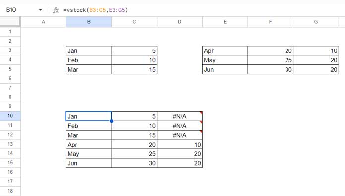
The following VSTACK formula appends those arrays vertically.
=vstack(B3:C5,E3:G5)While doing so, it finds which range, range1 or range2, contains the maximum number of columns and returns that many columns in the output.
So you may see #N/A errors in some cells. How do we remove them?
Replacing the #N/A in the VSTACK Result in Google Sheets
Since the number of columns in the range does not match, the above formula returns the default #N/A in some cells.
There is no pad_with argument similar to the WRAPCOLS or WRAPROWS functions in the VSTACK.
But we can use the IFERROR function to pad_with 0 (zero), blank, or some other values instead of the default value.
To replace #N/A in the VSTACK formula with zero, use the IFERROR as per the example below.
=iferror(vstack(B3:C5,E3:G5),0)Using Query in VSTACK and Blank Row Issue
You may encounter one issue when you want to vertically stack multiple Query results using the VSTACK function in Google Sheets.
You may get one or more blank rows or rows full of #N/A between the appended result.
It happens when one or more Query formulas fail to return any value that matches the criterion.
How to remove blank or error rows in VSTACK in Google Sheets?
We can name the VSTACK formula using LET and filter out blank rows.
Here is an example.
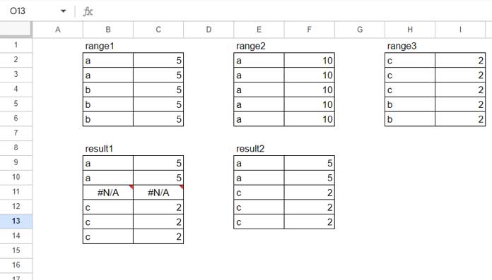
The range1, range2, and range3 are three Query formulas.
=vstack(query({B2:C6},"Select * where Col1='a'"),query({E2:F6},"Select * where Col1='b'"),query({H2:I6},"Select * where Col1='c'"))The second Query returns blank since the condition evaluates to FALSE.
The VSTACK formula leaves a row filled with #N/A in that case. Of course, we cause IFERROR to pad with blank.
=iferror(vstack(query({B2:C6},"Select * where Col1='a'"),query({E2:F6},"Select * where Col1='b'"),query({H2:I6},"Select * where Col1='c'")))But that may leave a blank row.
How to remove such blank rows in a VSTACK result in Google Sheets?
In the following formula, I’ve named the VSTACK with “blank” and filtered out the blank row.
=let(blanks,iferror(vstack(query({B2:C6},"Select * where Col1='a'"),query({E2:F6},"Select * where Col1='b'"),query({H2:I6},"Select * where Col1='c'"))),filter(blanks,index(blanks,0,1)<>""))That’s all about how to use the VSTACK function in Google Sheets.
Thanks for the stay. Enjoy!