Learn to apply date criteria in the FILTER function in Google Sheets.

In Google Sheets, in addition to the popular Filter command (Data > Create a filter), there is a FILTER function.

I always think functions have an edge over commands, and the FILTER function is an example of this.

In Google Sheets, functions typically offer more flexibility and advanced functionality compared to commands. The FILTER function, for example, allows for more complex filtering criteria and can be combined with other functions to achieve specific tasks, whereas commands may have more limited capabilities.

However, if you want to apply the filter directly to the source data, then the menu command, converting a range to a table (which adds a filter to the header), and Slicer are the best options.

Before going to the tutorial, if you wish to know the advantages of the FILTER function over the Filter command, go to my earlier post, Filter Data to Separate Sheets with Links. This is never possible with the Filter menu command.

Applying Date Criteria in the FILTER Function

To effectively filter a data range based on specific dates or date ranges, it’s crucial to understand how to correctly implement the date criteria.

It is easier if you refer to a cell, but hardcoding dates within the formula could affect the filtering if you incorrectly specify the date format.

Furthermore, you might want to use comparison operators or the function ISBETWEEN. We will see all these with a few examples below.

First, let’s look at the syntax of the function.

Syntax: FILTER(range, condition1, [condition2, …])

In this syntax, the range parameter represents the data range to filter, and the other parameters are conditions that are evaluated as TRUE or FALSE.

The Correct Way to Apply the Date Criteria in the FILTER Function

When hardcoding date criteria in the FILTER function, I suggest using the DATE function to specify the criterion.

The syntax is DATE(year, month, day).

Here are examples of using conditions:

A2:A = DATE(2024, 01, 15) – This condition will evaluate to TRUE wherever the date in column A equals January 15, 2024, and FALSE otherwise. When applying this condition, the FILTER function will filter the rows in the range wherever the condition evaluates to TRUE.

ISBETWEEN(A2:A, DATE(2024, 01, 01), DATE(2024, 01, 31)) – This will evaluate to TRUE wherever the dates in column A fall between January 1, 2024, and January 31, 2024. It adheres to the ISBETWEEN syntax: ISBETWEEN(value_to_compare, lower_value, upper_value, [lower_value_is_inclusive], [upper_value_is_inclusive]).

In the above case, you can specify two conditions using comparison operators:

• Condition1: A2:A >= DATE(2024, 01, 01)
• Condition2: A2:A <= DATE(2024, 01, 31)

Using these conditions in the FILTER function will help you correctly apply date criteria to filter your data.

Formula Examples

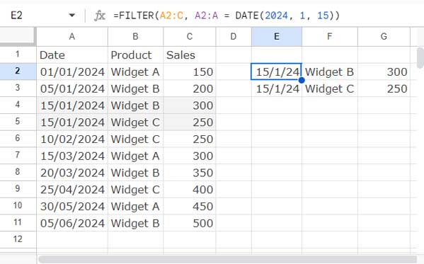
The following formula filters A2:C if A2:A is equal to January 15, 2024.

=FILTER(A2:C, A2:A = DATE(2024, 1, 15))

Instead of hardcoding the criterion, enter it in any blank cell outside the range and refer to that.

=FILTER(A2:C, A2:A = E1)

In this formula, E1 contains 15/01/204 in the same format as the criterion column, which is A2:A.

The following two formulas filter B2:C if A2:A is greater than or equal to January 1, 2024, and less than or equal to January 31, 2024.

=FILTER(B2:C, ISBETWEEN(A2:A, DATE(2024, 1, 1), DATE(2024, 1, 31)))
=FILTER(B2:C, A2:A >= DATE(2024, 1, 1), A2:A <= DATE(2024, 1, 31))

Common Date Criteria Issues in FILTER Function

The most common issue affecting filtering is incorrect date formatting.

To determine the correct format, add a new sheet by clicking the + button at the bottom left corner of the sheet and insert the formula =EOMONTH(TODAY(), 0) in cell A1 in that newly added sheet.

This will display the end-of-month date of the current month. From this, you can ascertain whether the date formatting should be MM/DD/YYYY, DD/MM/YYYY, or another suggested format like YYYY-MM-DD. You can follow this format when entering data.

If the dates in the criteria range are formatted as text, the FILTER function will fail. In such cases, you can wrap the criteria range with the DATEVALUE function as follows:

=FILTER(A2:C, DATEVALUE(A2:A) = E1)

These are the most common date criterion issues you may encounter when using the FILTER function in Google Sheets.

Resources

• How to Use AND, OR with Google Sheets Filter Function – Advanced Use
• Comma-Separated Values as Criteria in Filter Function in Google Sheets
• One Filter Function as the Criteria in Another Filter Function in Google Sheets
• IF Statement within Filter Function in Google Sheets
• How to Hardcode DATETIME Criteria within FILTER Function in Google Sheets
• IMPORTRANGE Within FILTER Function in Google Sheets
• Using HYPERLINK with FILTER Function in Google Sheets