You may need to sum every alternate column in Google Sheets when you have other numeric data in the columns in between. For this, you can use different formula options, and here are some dynamic ones.

You can use the following formula to sum every alternate column in a row in Google Sheets:

=SUM(FILTER(row, MOD(SEQUENCE(1, COLUMNS(row)), 2)=1))

In this formula, replace ‘row’ with the row reference you want.

If you want to repeat the calculation for every row, you can use another formula:

=ARRAYFORMULA(MMULT(IF(MOD(SEQUENCE(1, COLUMNS(range)), 2)=1, N(range), 0), TOCOL(COLUMN(range)^0)))

In this formula, replace ‘range’ with the range you want to apply the formula to.

Let’s look at two examples applying these formulas.

Example of Summing Every Alternate Cell in a Row in Google Sheets

In the following example, I have the gross and net salaries of a few employees, where the data range is A1:I6, with the header rows in A1:I2. The first column contains the employee names. The gross salaries for quarters Q1 to Q4 are in the ranges B3:B6, D3:D6, F3:F6, and H3:H6.

To sum the gross salaries in the first row, you can use the following formula in cell J3:

=SUM(FILTER(B3:I3, MOD(SEQUENCE(1, COLUMNS(B3:I3)), 2)=1))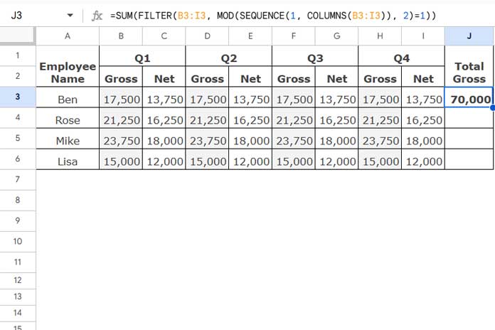

Drag this down to apply it to every row in the range.

If you want to sum the net salaries in every alternate column, use this formula instead:

=SUM(FILTER(B3:I3, MOD(SEQUENCE(1, COLUMNS(B3:I3)), 2)=0))

Here, the FILTER function filters the cells in B3:I3 wherever the condition is TRUE. In the first formula, the condition is:

MOD(SEQUENCE(1, COLUMNS(B3:I3)), 2)=1

The MOD function returns 1 for every alternate cell starting from B3. The values in between will be 0.

In the first formula, the condition evaluates to TRUE wherever the MOD function returns 1. In the second formula, the condition evaluates to TRUE where the MOD function returns 0.

Example of Summing Every Alternate Column in a Range in Google Sheets

In the previous example, we dragged the formula down the row to apply it to all rows. Instead, you can convert it into an array formula using the BYROW function as follows:

=BYROW(B3:I6, LAMBDA(row, SUM(FILTER(row, MOD(SEQUENCE(1, COLUMNS(row)), 2)=1))))

In this case, we converted the earlier formula into a custom LAMBDA function:

LAMBDA(row, SUM(FILTER(row, MOD(SEQUENCE(1, COLUMNS(row)), 2)=1)))

We then used this within the BYROW lambda helper function to apply it to each row in the specified range.

Note: Replace =1 with =0 depending on whether you want to sum every alternate column starting from the first column or from the second column in the range.

Alternatively, you can use the following formula:

=ARRAYFORMULA(MMULT(IF(MOD(SEQUENCE(1, COLUMNS(B3:I6)), 2)=1, N(B3:I6), 0), TOCOL(COLUMN(B3:I6)^0)))

This sums the gross salary columns. To sum the net salary columns, replace =1 with =0:

Here, we also use the MOD function to return 1 for every alternate column starting from the first column, and 0 for the columns in between.

The IF function evaluates whether the MOD function returns 1. If TRUE, it returns the numeric values from that column; otherwise, it returns 0.

We used this as Matrix 1 in the MMULT function, where Matrix 2 is a column with the number 1, matching the number of columns in the range. This will return column-wise sums in Google Sheets.

Resources

• How to Flatten Every Other Column in Google Sheets
• Vlookup on Every Other Column in Google Sheets
• How to Sum Every Nth Row or Column in Google Sheets
• How to Highlight Every Nth Row or Column in Google Sheets
• How to Copy Every Nth Cell from a Column in Google Sheets
• Dynamic Formula to Select Every Nth Column in Query in Google Sheets
• INDEX MATCH Every Nth Column in Google Sheets