


")


")

")
")
 in Excel & Google Sheets")


Most reports in Google Sheets break data into months or into calendar weeks (like Monday–Sunday). But sometimes, you need a different view — totals by week of the month. This isn’t as common, yet it’s extremely useful in scenarios like sales reporting (Week 1 vs. Week 2 performance), payroll cycles, or expense tracking.
Since Google Sheets doesn’t have a built-in function for “week of the month,” we’ll build it with formulas. In this tutorial, you’ll learn two powerful methods:
- SUMIFS → to calculate totals for a specific week in a given month.
- QUERY → to create a structured report summarizing all weeks of the month.
We’ll also use helper functions like DAY, ROUNDUP, and EOMONTH to assign dates to the correct week. Once set up, these formulas update automatically as you add more data.
What Does “Week of the Month” Mean?
Google Sheets doesn’t provide a built-in function to return the week of the month directly. Instead, we define it like this:
- Week 1 → Dates from the 1st to the 7th of the month
- Week 2 → Dates from the 8th to the 14th
- Week 3 → Dates from the 15th to the 21st
- Week 4 → Dates from the 22nd to the 28th
- Week 5 → Dates from the 29th to the end of the month (short week if the month has fewer than 31 days)
For example, in January 2025:
- Jan 1–7 → Week 1
- Jan 8–14 → Week 2
- Jan 15–21 → Week 3
- Jan 22–28 → Week 4
- Jan 29–31 → Week 5
Since this logic isn’t automatic, we’ll use formulas with DAY, ROUNDUP, and EOMONTH to calculate week numbers. Then we can easily sum values using SUMIFS or QUERY.
Sample Data for Summing by Week of the Month
To demonstrate, let’s assume the following dataset in A1:B:
| Date | Amount |
|---|---|
| 1/12/2024 | 6 |
| 2/12/2024 | 5 |
| 3/12/2024 | 8 |
| 4/12/2024 | 5 |
| 5/12/2024 | 10 |
| 6/12/2024 | 5 |
| … | … |
- Column A → Dates
- Column B → Amounts
Sum Data by Week of the Month Using SUMIFS
If you want to sum data for a specific week in a month, the SUMIFS function works best.
Step 1. In cell D2, enter the start date of the target month (e.g., 01/12/2024).
- To make this easier to read, format the cell as MMM YYYY:
- Select D2.
- Go to Format > Number > Custom number format.
- Enter
MMM YYYYand click Apply.
Now the date will show as Dec 2024 instead of01/12/2024.
Step 2. In cell E2, enter the week number (e.g., 1 for Week 1).
Step 3. Enter this formula in F2:
=ArrayFormula(SUMIFS(
  $B$2:$B,
  ROUNDUP(DAY($A$2:$A)/7), E2,
  EOMONTH($A$2:$A, -1)+1, D2
))
How the SUMIFS Formula Works
ROUNDUP(DAY($A$2:$A)/7)→ assigns each date to its week number within the month.EOMONTH($A$2:$A, -1)+1→ gives the first day of the month for each date.SUMIFS(...)→ filters rows by both month start (D2) and week number (E2), then sums the matching amounts.
👉 To get totals for Week 3, just change E2 to 3.
Sum Data by Week of the Month Using QUERY
If you prefer a report-style summary for all weeks in a month, QUERY is more efficient.
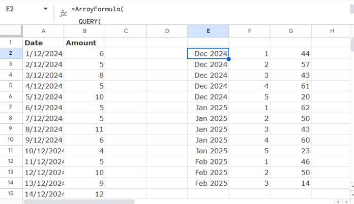
Use this formula (leave three empty columns for output expansion):
=ArrayFormula(
  QUERY(
    HSTACK(
      EOMONTH(A2:A, -1)+1,
      ROUNDUP(DAY(A2:A)/7),
      B2:B
    ),
    "SELECT Col1, Col2, SUM(Col3)
     WHERE Col1 IS NOT NULL
     GROUP BY Col1, Col2
     LABEL SUM(Col3) ''
     FORMAT Col1 'MMM YYYY'",
    0
  )
)
How the QUERY Formula Works
HSTACK(...)→ combines three helper columns:- Start of the month
- Week number within the month
- Amount values
QUERY(...)→ groups by month + week number and calculates sums.FORMAT Col1 'MMM YYYY'→ displays month and year cleanly.
👉 The result is a table summarizing totals for every week in each month.
Conclusion
Summing data by week of the month in Google Sheets helps you analyze trends more precisely than looking at full months.
- Use SUMIFS if you need to target one week at a time.
- Use QUERY if you want a complete summary report of all weeks.
With helper functions like DAY, ROUNDUP, and EOMONTH, you can calculate week numbers easily and keep your reports dynamic.