If you have a list of durations in seconds and want to display them in a readable HH:MM:SS format, Google Sheets makes it easy with a formula that returns an actual time value—not plain text.
This means you can still sort, filter, and perform calculations with the result. Whether you’re tracking time for workouts, video clips, or task durations, converting seconds into hours, minutes, and seconds will make your data more useful and understandable.
In this tutorial, I’ll show you how to convert seconds to HH:MM:SS in Google Sheets, step by step.
Formula to Convert Seconds to Time in the Format HH:MM:SS in Google Sheets
To convert seconds to time in Google Sheets, use the following formula:
=QUERY(MOD(A1/86400, 1), "SELECT Col1 FORMAT Col1 'hh:mm:ss'")- Replace
A1with the cell reference containing your duration in seconds.
If the value in A1 is greater than or equal to 86,400 (the number of seconds in a day), you may also want to calculate the day component separately using:
=TRUNC(A1/86400)This will return the number of full days in the given duration.
We’ll go over how this formula works after a few practical examples.
Examples of Converting Seconds to Time
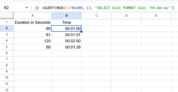
Assume you have the following durations in column A (starting from cell A2):
| Duration in Seconds |
| 60 |
| 61 |
| 120 |
| 88 |
To convert these seconds to HH:MM:SS in Google Sheets, enter the following formula in cell B2 and drag it down:
=QUERY(MOD(A2/86400, 1), "SELECT Col1 FORMAT Col1 'hh:mm:ss'")Your output in column B will look like this:
Optionally, if you want to extract the day component (in case some durations are longer than 24 hours), enter the following formula in cell C2 and drag it down:
=TRUNC(A2/86400)For example, if the value in A2 is 150000 seconds, the formulas would return:
- Time (
QUERY):17:40:00 - Days (
TRUNC):1
How Does the Formula Work?
Let’s break it down:
A2/86400
Divides the seconds by the number of seconds in a day (86,400) to get the equivalent duration as a decimal fraction of a day.MOD(A2/86400, 1)
Strips out the integer part (days), leaving only the decimal part which represents the time of day.QUERY(..., "SELECT Col1 FORMAT Col1 'hh:mm:ss'")
Converts the decimal value to theHH:MM:SStime format while keeping it as a valid time value (not plain text). We useQUERYinstead ofTEXTto maintain a time-formatted number that remains usable in further calculations.
This method is especially useful if you want to perform additional operations on the time values, such as adding durations or comparing times.
Related Resources
- Round, Round Up, and Round Down Hours, Minutes, and Seconds in Google Sheets
- How to Add Hours, Minutes, Seconds to Time in Google Sheets
- How to Format Time to Milliseconds in Google Sheets
- How to Convert a Timestamp to Milliseconds in Google Sheets
- How to Remove Milliseconds from Timestamps in Google Sheets


