Summary:
Learn how to find running minimum values (cumulative minima) in Google Sheets using non-array formulas like MIN, or array formulas like SCAN and DMIN. This tutorial covers step-by-step methods for stock prices, cumulative minimum logic, and even a legacy approach using DMIN.

Let’s learn how to find running minimum values, also called cumulative minima or cumulative minimum, using array and non-array formulas in Google Sheets.

We can use non-array MIN, or array formulas like DMIN and the new SCAN to calculate cumulative minima in Google Sheets.

If you invest in stocks, you may find these formulas particularly useful.

Using them, you can easily find how far a particular or current price point is from the historical minimum throughout the day.

For example:

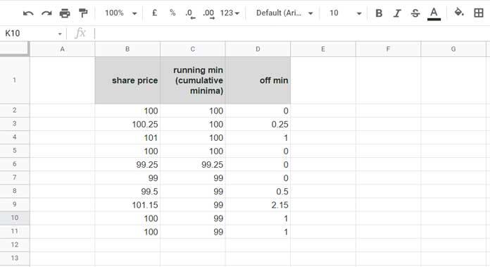
I have the share price of an automotive manufacturing company throughout the day in an array (B2:B11) in Google Sheets.

The running minimum values are in C2:C11, and how far off the share price is from the cumulative minima at each point is in D2:D11.

Note: To find cumulative maxima, you can use MAX, DMAX, or SCAN formulas. I have detailed that here: Running Max Values in Google Sheets (Array Formula Included).

What Are the Formulas Used in Cells C2 and D2?

Finding Running Minimum Values (aka Cumulative Minima) in Google Sheets

Here we go!

Cumulative Minimum Using MIN (Non-Array Formula)

In cell C2, insert the following MIN formula and drag it down:

=MIN($B$2:B2)

For cell D2, use:

=B2-C2

And drag it down as well.

SCAN Array Formula to Get Running Minimum Value in Google Sheets

The new SCAN function is the best array solution to get running minimum values in Google Sheets.

We usually use it for running sums, but here we’ll apply it to cumulative minimums. It processes an initial value (accumulator) row by row through the array.

Syntax: SCAN(initial_value, array_or_range, lambda)

Before using SCAN for this, it’s important to understand what cumulative minimum (Cummin) means.

Cummin is simply comparing the current value with the previous minimum and keeping the smaller one.

Cummin Array Formula for C2:

=SCAN(B2, B2:B, LAMBDA(a, v, IF(a <= v, a, v)))

Logic:

• The initial_value (a) is the first value in the array.
• In the first row, since a and v are the same, it returns that value.
• From the second row onwards, it compares the previous minimum (a) with the current value (v) and returns the smaller one.
• This logical test a <= v continues for every row.

You can also find how far the share price is from the cumulative minima using an array formula:

In D2, insert:

=ArrayFormula(IF(LEN(B2:B), B2:B-C2:C, ))

Legacy Method: Using DMIN for Running Minimum (Before SCAN)

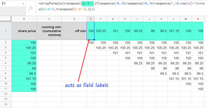
Suppose you have a 10-by-1 vector of share prices in the range B2:B11.

How do you use DMIN to find the running minimum?

Let’s break it down step-by-step:

Logic Behind Finding Cumulative Minima with DMIN

We have a 10-row, 1-column matrix (B2:B11).

We need to transform it into a 10×10 matrix (10 rows × 10 columns) so we can compute the minimum of each column individually.

By doing so, we find the cumulative minimum through an array formula.

Two steps involved:

1. Transform Data to 10×10 Matrix
2. Apply DMIN to Each Column

Step 1: Transforming Data

In E1, insert:

=ARRAYFORMULA(TRANSPOSE({B2:B11, IF(SEQUENCE(10, 10) / SEQUENCE(10, 10) + SEQUENCE(1, 10, ROW(A2)-1)<=ROW(A2:A11), TRANSPOSE(B2:B11),)}))

This will create the database for the DMIN operation.

Step 2: Cumulative Minimum Using DMIN Array Formula

In C2, use:

=ARRAYFORMULA(DMIN(E1:N11, SEQUENCE(10), {IF(,,); IF(,,)}))

• The SEQUENCE function generates numbers 1 to 10, corresponding to field IDs in the DMIN database.

Then, replace E1:N11 with the full transformed array formula from Step 1 to make it dynamic.

Final cumulative minima formula:

=ARRAYFORMULA(DMIN(TRANSPOSE({B2:B11, IF(SEQUENCE(10, 10) / SEQUENCE(10, 10) + SEQUENCE(1, 10, ROW(A2)-1)<=ROW(A2:A11), TRANSPOSE(B2:B11),)}), SEQUENCE(10), {IF(,,); IF(,,)}))

Closed vs. Open Ranges

I’ve modified the formula accordingly in my sample sheet below.

Sample Sheet

Resources

• How to Average the Lowest N Numbers in Google Sheets
• How to Exclude Zeros from MIN Function Results in Google Sheets
• Using MIN in Arrays in Google Sheets: A Complete Guide
• Finding Max and Min Values in GoogleFinance Historical Data in Sheets
• Min in Vlookup in Google Sheets – Formula Examples
• Find the Column Header of the Min Value in Google Sheets
• Get Min Date Ignoring Blanks in Each Row in Google Sheets
• Max and Min Strings Based on Alphabetic Order in Google Sheets
• Find and Filter the Min or Max Value in Groups in Google Sheets
• Lookup the Smallest Value in a 2D Array in Google Sheets
• How to Find All Lowest-Priced Items in Google Sheets