


Row-wise sorting is the process of sorting each row in a 2-D array using an array formula in Google Sheets. We can do this using the BYROW or REDUCE functions with the SORT function. The QUERY function can also be used, but it is not recommended because it can be more complex for some users.
Here is an example of row-wise sorting a 2-D array in Google Sheets:
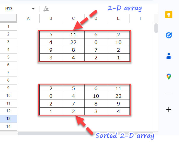
The source data is in the range B2:E5, and the result is in the range B9:E12.
We can easily handle this using a non-array formula (a copy-paste or drag-down formula) in Google Sheets. However, I would rather use an array formula since the source data may not always be physical. It can also be an expression such as the output of the QUERY or some other functions.
However, for those of you who would like to see the non-array formula for sorting each row individually in a 2D array, here it is:
=TRANSPOSE(SORT(TRANSPOSE(B2:E2),1,1))Note: To sort rows in descending order replace 1 with 0.
Insert the above formula in cell B9 and copy-paste it into B10:B12. Alternatively, you can drag the B9 fill handle (a small blue square in the bottom right corner) down.
Related: How to Sort Horizontally in Google Sheets.
We will convert this into an array formula, and I will explain the role of TRANSPOSE in the process.
Row-Wise Sorting in a 2-D Array: BYROW
Let’s start by using BYROW, which is my recommended solution to row-wise sorting of a 2D array in Google Sheets.
In the above example, we have a 2D array in the range B2:E5 and can sort each row of this array in ascending order by using the following array formula in cell B9.
=BYROW(B2:E5,LAMBDA(row,TRANSPOSE(SORT(TRANSPOSE(row),1,1))))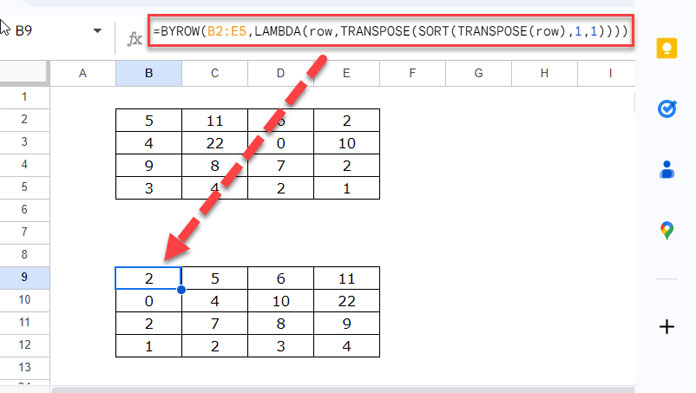
You are not restricted to entering the formula in cell B9. The thumb rule is to enter the formula in any cell and give it enough room (blank cells) to expand down and to the right.
If you want row-wise sorting in descending order, use this one.
=BYROW(B2:E5,LAMBDA(row,TRANSPOSE(SORT(TRANSPOSE(row),1,0))))The difference is negligible, which you can see from the formulas themselves.
How does this formula work?
BYROW Syntax:
BYROW(array_or_range, lambda)The BYROW function applies a lambda to each row in the array_or_range and returns an array of the results.
array_or_range:B2:E5(it will be separated by rows such as B2:E2, B3:E3, B4:E4, and B5:E5).lambda: Please refer to the syntax below.
LAMBDA Syntax: LAMBDA([name, …], formula_expression)
name:row(which represents the row in thearray_or_range).formula_expression:TRANSPOSE(SORT(TRANSPOSE(row),1,1))
This formula_expression first TRANSPOSEs the row, then SORTs the transposed row, and then TRANSPOSEs the sorted row again. This applies to each row in the array_or_range.
Additional Tip
We can also use the TOCOL and TOROW functions instead of the TRANSPOSE function in the formula_expression part. Here is the formula expression:
TOROW(SORT(TOCOL(row), 1, 1))This formula expression first TOCOLs the row, then SORTs the TOCOLed row and then TOROWs the sorted row again.
The TOCOL function converts a range of cells into a single column, while the TOROW function converts a range of cells into a single row.
By using the TOCOL and TOROW functions, we can avoid having to use the TRANSPOSE function twice. This can make the formula more concise and easier to understand.
I hope the above explanation has helped you understand how to use the BYROW function for row-wise sorting in a 2D array in Google Sheets.
Row-Wise Sorting in a 2-D Array: REDUCE
Though I prefer the above BYROW approach for row-wise sorting of a 2D array, you can also use the REDUCE function for the same.
Note: This is just to help you learn more about the advanced use of REDUCE in Google Sheets.
Formula:
=REDUCE(,SEQUENCE(ROWS(B2:E5)),LAMBDA(a,v,IFNA(VSTACK(a,TOROW(SORT(TOCOL(CHOOSEROWS(B2:E5,v))))))))It has two drawbacks, not in terms of performance, but in terms of coding and output.
- It is more complex to code than the BYROW approach.
- It returns an empty row at the top of the result.
Can you explain how this formula performs row-wise sorting in Google Sheets?
Yes. Here is the structure of the formula.
REDUCE Syntax:
REDUCE(initial_value, array_or_range, lambda)intial_value: null
array_or_range: SEQUENCE(ROWS(B2:E5)) (serial numbers 1 to 4 represent the rows in the range B2:E5).
lambda: Please see the syntax below.
LAMBDA Syntax: LAMBDA([name1, name2], formula_expression)
name1:awhich represents the accumulator (the accumulated value in each step).name2:vwhich represents the row in thearray_or_range.formula_expression:IFNA(VSTACK(a,TOROW(SORT(TOCOL(CHOOSEROWS(B2:E5,v))))))
The VSTACK function vertically stacks the accumulator (which is initially null) with the following: TOROW(SORT(TOCOL(CHOOSEROWS(B2:E5,v))))
What does it do?
The CHOOSEROWS function in the formula expression returns the first row of the array. The TOCOL function converts the row to a column. The SORT function sorts the column. The TOROW function transforms the sorted column back into a row.
The array is passed to the accumulator.
This process repeats for each row in the array. The final accumulator value, which is returned by the formula, is a row-wise sorted 2D array.
To put it simply, the formula takes the first row of the array, sorts it, and then adds it to the accumulator. This process repeats for each row in the array, and the final accumulator value is a row-wise sorted 2D array.
That’s all. Thanks for the stay. Enjoy!