


")


")

")
")
 in Excel & Google Sheets")


This post explains how to create a rolling months summary report in Google Sheets.
In such a summary, you can use aggregation functions like SUM, AVERAGE, COUNT, MAX, MIN—or even all of them.
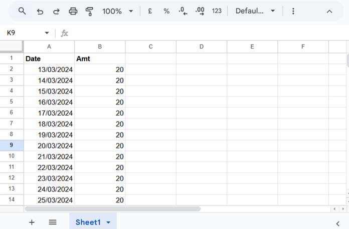
To build a rolling months summary in Google Sheets, you’ll need at least two columns:
- A date column
- A number column
My sample data contains over 500 rows, so it’s not practical to include a full screenshot or display the data as a table here. Below is a partial snapshot for a quick glance:
Also, there’s another reason I haven’t shared the full dataset:
Since this summary is based on rolling months, the current date plays a critical role. That means the sample data may not work correctly for you if viewed at a later date.
To recreate the sample data yourself, you can use the following formula in cell A2 to generate a rolling date range:
=SEQUENCE(
  DAYS(TODAY(), TODAY()-500) + 1,
  1,
  TODAY()-500
)
Then fill the adjacent column (B2:B) with random numbers to simulate actual data.
Introduction to Rolling Months
Assume today’s date is 26 July 2025.
- All dates in June 2025 will be grouped under Rolling Month 1
- May 2025 will be Rolling Month 2
- April 2025 will be Rolling Month 3, and so on.
In short:
Rolling X Months typically refers to the X most recent complete calendar months—a preferred approach in reporting since it avoids inconsistencies caused by partial months.
Now that we understand the logic, let’s see how to assign rolling month numbers to a list of dates in Google Sheets.
How to Assign Rolling Month Numbers in Google Sheets
Let’s start with assigning month numbers that represent their position in the rolling window.
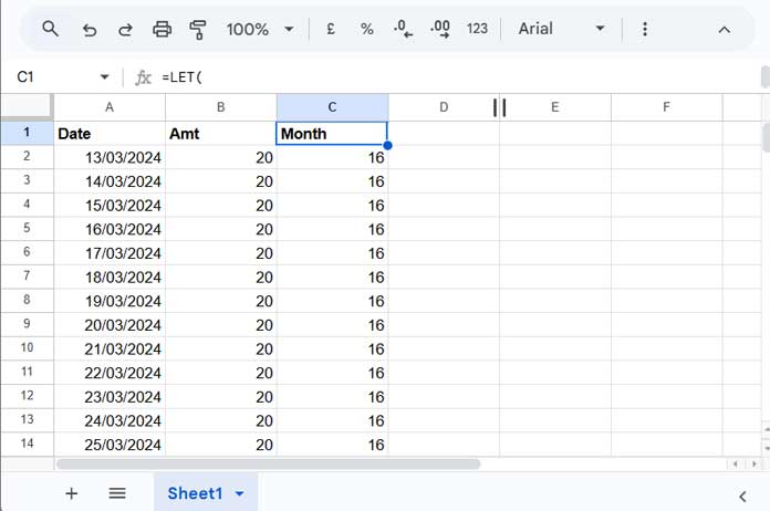
Assume your dates start in cell A2 under column A, with A1 as the header. In cell C1, enter the following formula:
=LET(
  date_range, A2:A,
  header, "Month",
  months, ARRAYFORMULA(IFERROR(DATEDIF(EOMONTH(date_range, -1)+1, EOMONTH(EDATE(TODAY(), -1), 0), "m") + 1)),
  VSTACK(header, months)
)
This formula outputs rolling month numbers in column C, with the header “Month” in cell C1 and the month numbers starting from C2.
Formula Breakdown
The core of the formula is:
ARRAYFORMULA(IFERROR(DATEDIF(EOMONTH(date_range, -1)+1, EOMONTH(EDATE(TODAY(), -1), 0), "m") + 1))Which follows this structure:
DATEDIF(start_date, end_date, "m") + 1It calculates the number of full months between a given start and end date, and adds 1. The +1 ensures the most recent completed month is Month 1, not 0.
Explanation
- Start date:
EOMONTH(date_range, -1) + 1
This gives the first day of the month for each date in column A.
For example, if a date is 20 June 2025, the start date becomes 01 June 2025. - End date:
EOMONTH(EDATE(TODAY(), -1), 0)
This returns the last day of the most recent completed month.
IfTODAY()is 26 July 2025, the end date will be 30 June 2025. - DATEDIF:
DATEDIF(start_date, end_date, "m")
Returns the number of full months between the two dates.
For example:DATEDIF("01/06/2025", "30/06/2025", "m")returns0→ we add1to get1.
As a result, the formula assigns:
1for the most recent completed month2for the previous month3for two months ago, and so on
Generate a Rolling Months Summary in Google Sheets Using QUERY
Now that we’ve completed the tricky part—assigning rolling month numbers—we can use the QUERY function to generate the Rolling Months Summary in Google Sheets.
Here’s a basic example that summarizes values over the last 3 months:
=QUERY(A1:C, "SELECT Col3, SUM(Col2) WHERE Col3>=1 AND Col3<=3 GROUP BY Col3", 1)This creates a rolling 3-month summary as follows:
| Month | sum Amt |
| 1 | 323 |
| 2 | 301 |
| 3 | 358 |
You can adjust the condition (Col3 <= 3) to generate summaries for different periods:
- For a rolling 1-month summary: change to
Col3 <= 1 - For 12 months: change to
Col3 <= 12
Handling More Columns in the QUERY Summary
If your dataset has three columns (for example: Date, Value, and Category), place the helper formula in column D starting at cell D1. In that case, update your QUERY range to A1:D and adjust the column references accordingly:
=QUERY(A1:D, "SELECT Col4, SUM(Col2) WHERE Col4>=1 AND Col4<=3 GROUP BY Col4", 1)You can also replace SUM(Col2) with other aggregation functions:
AVG(Col2)– AverageCOUNT(Col2)– CountMIN(Col2)– MinimumMAX(Col2)– Maximum
Or combine them:
=QUERY(A1:D, "SELECT Col4, SUM(Col2), COUNT(Col2), AVG(Col2), MIN(Col2), MAX(Col2) WHERE Col4>=1 AND Col4<=3 GROUP BY Col4", 1)This returns a detailed rolling months summary in Google Sheets that includes multiple metrics per month.
| Month | sum Amt | count Amt | avg Amt | min Amt | max Amt |
| 1 | 323 | 30 | 10.77 | 10 | 11 |
| 2 | 301 | 31 | 9.71 | 9 | 10 |
| 3 | 358 | 30 | 11.93 | 9 | 20 |