With the help of the RegexReplace function, we can easily wrap numbers in a text string in brackets in Google Sheets.

This we can use to format the strings containing numbers. Other than this, there is one important use of adding brackets around numbers in Google Sheets.

As (partially) mentioned in the title, we can use the above Regex method to dynamically refer columns when using aggregation functions in Query.

You May Like: How to Sum, Avg, Count, Max, and Min in Google Sheets Query.

Let’s start this tutorial with how to use RegexReplace to wrap numbers in brackets in Google Sheets. The Query comes after that.

How to Add Brackets Around Numbers Using the RegexReplace Function in Google Sheets?

In my example below, I am using parentheses to wrap around the numbers. Instead, you can use square brackets too.

Syntax:

REGEXREPLACE(text, "(\d+)", "($1)")

Example 1:

The content of cell B2 is the text Purchase 100, Damage 50. The following RegexReplace formula in cell B3 will return the result; Purchase (100), Damage (50).

=REGEXREPLACE(B2,"(\d+)", "($1)")

To replace the parentheses around the numbers with square brackets, use the below formula.

=REGEXREPLACE(B2,"(\d+)", "[$1]")

See one more example.

Example 2:

This time the value in cell B2 is the number 100.

Here the above formula won’t work as the content in cell B2 doesn’t contain any text string!

You must use B2&"" instead of B2 to convert the number in cell B2 to text because RegexReplace is a text function and only takes text as the argument 1.

=REGEXREPLACE(B2&"","(\d+)", "[$1]")

This way we can use the RegexReplace function to wrap numbers in brackets in Google Sheets.

I have found one important use, or we can say real-life use, of this formula in the Query function. Let’s go to that.

RegexReplace to Wrap Numbers in Brackets and Its Query Select Clause Use

You have just learned how to use the RegexReplace function to wrap numbers in parenthesis (brackets) in Google Sheets.

Now let’s see how to use it in Query Select clause to dynamically refer to columns in Query aggregation functions.

Query Function ‘query’ – Non-Dynamic

Please see the image below for the sample data.

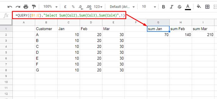
With the help of the Sum aggregation function in Query, we can sum the columns C, D, and E (Columns 2, 3 and 4 in the range B1:E).

=QUERY({B1:E},"Select Sum(Col2),Sum(Col3),Sum(Col4)",1)

This normal Query formula has one drawback!

To know that, insert one column before column E. Only the range B1:E (data) will be automatically get adjusted within the formula.

Syntax: QUERY(data, query, [headers])

The ‘query’ argument is actually entered as a string (within double quotes). So it won’t get adjusted when the ‘data’ range changes.

Here I am going to make the ‘query’ argument dynamic with the help of our above RegexReplace formula.

Query Function ‘query’ – Dynamic

Here is the ‘query’ non-dynamic syntax.

"Select Sum(Col2),Sum(Col3),Sum(Col4)"

Using the below Sequence formula we can generate the column numbers to sum dynamically.

=sequence(1,columns(C1:E1),2)

The above Sequence formula in cell G1 adjusts based on new columns in the range.

Once again see the syntax of the RegexReplace formula that wraps numbers in brackets in Google Sheets. Here is that.

REGEXREPLACE(text, "(\d+)", "($1)")

In this, we need to replace/feed the ‘text’ argument with the above Sequence formula. But the Sequence formula output is a multi-column number. So it won’t work. Then?

As mentioned in the example 2, we must use &"" at the last part of the Sequence.

=REGEXREPLACE(sequence(1,columns(C1:E1),2)&"","(\d+)", "($1)")

Then wrap it with ArrayFormula since there is an array in use as ‘text’ in RegexReplace.

=ArrayFormula(REGEXREPLACE(sequence(1,columns(C1:E1),2)&"","(\d+)", "($1)"))

Output:

We have added brackets around numbers. I am slightly modifying the formula.

=ARRAYFORMULA(REGEXREPLACE(sequence(1,columns(C1:E1),2)&"","(\d+)", "Sum(Col$1)"))

Output:

Then TextJoin these outputs.

=TEXTJOIN(",",TRUE,ARRAYFORMULA(REGEXREPLACE(sequence(1,columns(C1:E1),2)&"","(\d+)", "Sum(Col$1)")))

Result:

Sum(Col2),Sum(Col3),Sum(Col4)

Now, finally in the Query formula, I am replacing the ‘query’ with the above formula.

=QUERY({B1:E},"Select "&TEXTJOIN(",",TRUE,ARRAYFORMULA(REGEXREPLACE(sequence(1,columns(C1:E1),2)&"","(\d+)", "Sum(Col$1)"))),1)

I hope you could learn the use of RegexReplace to wrap numbers in brackets and one of its real-life use with the help of Query.

Resources

• How to Restrict Entering Special Characters in Google Sheets Using Regex.
• Extract Username from Email Address Using Regex in Google Sheets.
• Regexmatch in Filter Criteria in Google Sheets [Examples].
• Match Two Columns that Contain Values Not in Any Order Using Regex.
• REGEXMATCH in SUMIFS and Multiple Criteria Columns in Google Sheets.
• Regex to Replace the Last Occurrence of a Character in Google Sheets.
• Regexmatch Dates in Google Sheets – Single/Multiple Match.
• Exact Match Using Regular Expression in Google Sheets.