


")


")

")
")
 in Excel & Google Sheets")


To pick random values based on conditions, we’ll use a combination of SORTN, FILTER, RANDARRAY, and COUNTIFS functions in Google Sheets. The key function here is RANDARRAY.
You could technically replace some of these functions—like using QUERY instead of FILTER, a combo of SORT and ARRAY_CONSTRAIN instead of SORTN, or COUNTIF instead of COUNTIFS. But in my opinion, the combination I’ve used is the most efficient and flexible way to pick random values with conditions in Google Sheets.
We’ll walk through two examples. The first one involves a single condition, while the second includes multiple conditions.
Example 1: Pick Random Values with a Condition in Google Sheets
Let’s consider the following sample dataset:
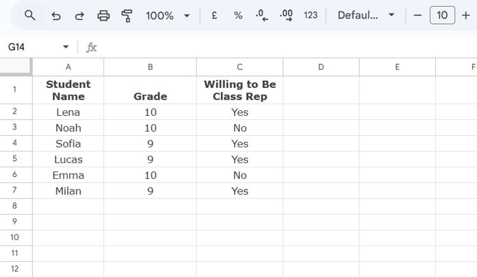
Suppose you have a list of students from different grades and want to randomly select two students who are willing to become the class representative.
That means, from column A (Student Name), you want to pick two random names where the last column says Yes.
Use this formula:
=SORTN(
   FILTER(A2:A, C2:C = "Yes"),
   2,
   0,
   RANDARRAY(COUNTIFS(C2:C, "Yes")), 1
)
Breakdown of the Formula:
FILTER(A2:A, C2:C = "Yes")– filters students who are willing to lead.COUNTIFS(C2:C, "Yes")– counts how many students are willing to lead.RANDARRAY(...)– generates that many random numbers.SORTN(...)– sorts the filtered names by the random numbers and returns 2 of them.
If you want to return 3 random names instead of 2, just change the second argument in SORTN to 3.
This is one of the simplest and cleanest ways to pick random values with a condition in Google Sheets.
Example 2: Pick Random Values with Multiple Conditions in Google Sheets
Now let’s apply two conditions.
Say you want to randomly select two students from Grade 9 who are also willing to be class representatives.
You can use the same formula pattern—just add the second condition to both FILTER and COUNTIFS:
=SORTN(
   FILTER(A2:A, B2:B = 9, C2:C = "Yes"),
   2,
   0,
   RANDARRAY(COUNTIFS(B2:B, 9, C2:C, "Yes")), 1
)
Make sure the conditions match in both FILTER and COUNTIFS.
This will return two random students who meet both conditions: Grade 9 and willing to lead.
What If There Are Fewer Than N Matching Rows?
You might wonder what happens if there are fewer qualifying students than the number you want to pick. For example, what if you want to pick 5 random students from Grade 9 who are willing to lead—but only 3 such students exist?
The formula will simply return the available rows. In this case, you’ll get 3 names.
But if there are no matching values, the formula will return a #NUM! error.
To avoid showing an error in such cases, just wrap the formula in IFERROR:
=IFERROR(SORTN(FILTER(...), ...))This will suppress the error and return a blank cell instead.