


In a nested Vlookup formula in Google Sheets, a Vlookup is written inside another Vlookup. The inner Vlookup will act as the search_key of the outer Vlookup.
When you nest Vlookup formulas in Google Sheets, you may normally face one issue. That will be the column order (position).
I know you didn’t get the point. Normally there will be a minimum of two tables involved in a nested Vlookup in Google Sheets.
If your inner Vlookup output (the search_key of the outer Vlookup) is not available in the first column of the outer Vlookup table, the formula will return #N/A error.
How to troubleshoot that problem?
This post contains the answer to the above problem too. Let’s start learning how to nest multiple Vlookup formulas in Google Sheets.
As a side note, for those who are new to Vlookup, check this – Vlookup in Google Sheets – How to and Formula Variations.
Nested Vlookup Examples in Google Sheets
Earlier I have handled a large set of data on the fuel consumption of heavy trucks and office cars. So I think, this time, for the explanation purpose, let me make an example from that.
Table 1: Vehicle and Driver
The range of the following table in my Sheet is Sheet1!B2:C7.
| Driver | Vehicle Number |
| Albert | 96D123 |
| Paul | 96A154 |
| Justin | 96F452 |
| Samuel | 95A100 |
| James | 95F011 |
Table 2: Vehicle and Fuel Consumption
Data Range is Sheet1!E2:F7
| Vehicle Number | Fuel Consumption in gal |
| 96D123 | 743.00 |
| 96A154 | 783.00 |
| 96F452 | 373.00 |
| 95A100 | 410.00 |
| 95F011 | 461.00 |
At this point, you may have one doubt whether the vehicle number on the two tables should be in the same order or not.
The answer is ‘NO’. I have just maintained the order to create two tables by copy-pasting the values.
Problem to Solve Using Nesting Two Vlookups
Find the fuel consumption of the vehicle driven by “Paul”.
That means there is only one search_key that is “Paul”.
Single Search_Key Values
Let’s solve the above Vlookup problem with the help of a nested Vlookup formula.
Take a look at the two tables. The fuel consumptions are in table 2 and the drivers’ names are in table 1.
Both the tables have one common column that is vehicle number.
So in the first Vlookup (inner Vlookup), we can use the driver name “Paul” as the search_key to find the vehicle number.
The table that contains the said pieces of information is table 1.
The following Vlookup formula will return the vehicle number “96A154” driven by the driver “Paul”.
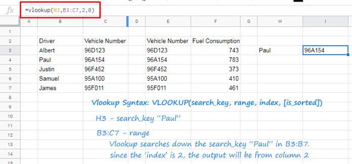
=vlookup("Paul",B3:C7,2,0)
or use;
=vlookup(H3,B3:C7,2,0)
For those who are not familiar with Vlookup, let me explain the formula with the help of an image.
Time to nest the Vlookup formula now. We have got the number of the vehicle driven by “Paul” which is “96A154”.
Use that (I mean the above Vlookup itself) as the search_key in another Vlookup. That’s called nesting.
This time we will use table 2 which contains the vehicle number and fuel consumption details.
Syntax of the Nested Vlookup Formula:
VLOOKUP(Vlookup_formula_as_search_key, range, index, [is_sorted])Here is our nested Vlookup formula to return the fuel consumption of the vehicle driven by “Paul”.
=vlookup(vlookup(H3,B3:C7,2,0),E3:F7,2,0)Result: 783.00
In this E3:E7 is the range of the second table. Column 1 in that table contains the vehicle number and column 2 contains the fuel consumption data.
Multiple Search_Key Values
Similar to regular Vlookup we can use multiple search_key values in a nested Vlookup too.
Related: How to Use Vlookup to Return an Array Result in Google Sheets.
Instead of one search_key, let’s use two search_keys in a nested Vlookup formula in Google Sheets.
The search_keys are “Paul” and “James”.
The changes will be in the inner Vlookup. Earlier the search_key was in cell F3. This time the search_keys are in F3:F4.
So change the search_key reference F3 to F3:F4 in the inner Vlookup. Additionally, wrap the outer Vlookpu with ArrayFormula function.
=ArrayFormula(vlookup(vlookup(H3:H4,B3:C7,2,0),E3:F7,2,0))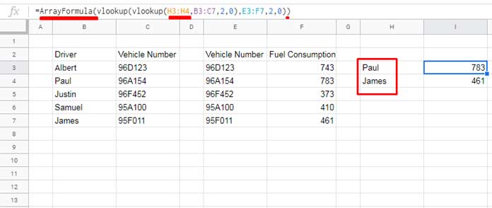
This way you can use nested Vlookup in similar scenarios including sales or financial data in Google Sheets.
Nested Vlookup – Search Column Other than First Column
In the beginning, I have mentioned one of the issues of Vlookup nesting. Here is that.
Since a nested Vlookup formula involves more than one Vlookup, sometimes the search_key column can cause an issue.
The reason Vlookup is famously known for search across the first column of a range.
See the two tables that contain some sample sales data.
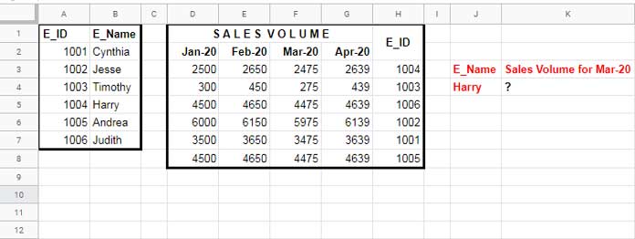
How to find the sales volume for the month of Mar-20. The salesperson’s name is “Harry” (Vlookup search_key).
Finding E_ID Using E_Name (Inner Reverse Vlookup)
Let’s write the inner Vlookup first. The following formula will definitely return #N/A! error as there is no value “Harry” in the first column of the range A2:A7.
Wrong Formula:
=vlookup(J4,A2:B7,1,0)So what’s the correct solution here?
If you have read my article titled Reverse Vlookup Examples in Google Sheets, you won’t struggle here much.
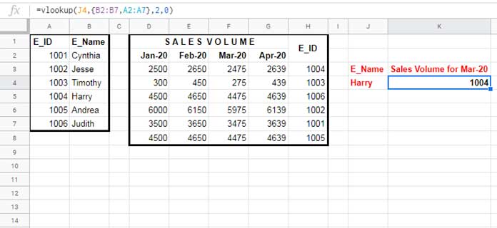
Correct Formula:
=vlookup(J4,{B2:B7,A2:A7},2,0)The Vlookup range A2:B7 modified as {B2:B7,A2:A7}. By doing so I have virtually moved the second column to first.
So we are ready with the inner Vlookup. Let’s start writing the nested Vlookup formula now.
Finding Sales Volume Using E_ID (Nested Reverse Vlookup in Google Sheets)
We have the E_ID of the employee “Harry” now. That means the search_key is the Vlookup above and the range is D3:H8.
But wait! Here again, we have to virtually shuffle the columns as the E_ID is in the last column.
We must move the last column to first and this will do that.
={H3:H8,D3:G8}Reverse Vlookup in Nesting (Formula):
=Vlookup(vlookup(J4,{B2:B7,A2:A7},2,0),{H3:H8,D3:G8},4,0)Result: 2475