You won’t believe you can do wonder with the Named Ranges in Sumif in Google Sheets. Let me shed some light on the use of Named Ranges in the Sumif, the conditional sum function.

The Sumif has the following arguments. They are the range, criterion, and sum_range. You can replace any of them with the Named Ranges.

The role of the Named Ranges in Sumif in Google Sheets varies depending upon the usage. I mean in which argument you are using it.

Before starting here is a quick introduction on how to use the Sumif function.

How to SUMIF in Google Sheets

I believe it’s my responsibility to first introduce you to the function Sumif. Then we can move to the use of Named Ranges in Sumif in Google Sheets.

I have already this function featured on many times on this site. Click on the search icon on the top navigation bar and type “Sumif” to find an impressive set of guides.

But to save your time here is a quick tutorial on how to Sumif in Google Sheets.

Syntax:

SUMIF(range, criterion, [sum_range])

Example:

Sample Data: Please scroll down and refer to the first screenshot for the sample data used in this example.

=sumif(A3:A8,"Road Base",C3:C8)

In concise, this formula explains how to Sumif in Google Sheets. This Sumif formula checks the range A3: A8 for the criterion “Road Base” and sum the values in the sum_range in the found row.

Named Ranges in Sumif in Google Sheets

Let me show you how to replace the range, criterion as well as sum_range in Sumif with Named Ranges.

I find the Named Ranges very useful in Sumif when using as sum_range. So I am beginning with that.

Named Ranges in Sumif – Replacing Sum_range

In my sample data below, there are three columns with numbers. They are Column C, D, and E. You can conditionally sum any of those columns using the Sumif in Google Doc Sheets.

I will share you one awesome Sumif Google Sheets tip now. See how to switch sum_range in Sumif with the help of a drop-down menu.

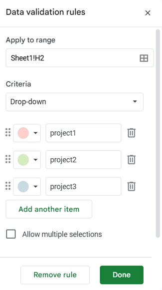
The drop-down menu in cell H2 contains three menu items – project1, project2, and project3.

Actually, these three text strings are representing the named ranges to C3: C, D3: D, and E3: E respectively.

Note:

1. You can create Named Ranges by selecting the cells that you want to name and then going to the menu Data > Named range.

2. You can find the drop-down menu creating option under the menu Data > Data Validation.

To create a drop-down menu here for the sum_range, Select the cell H2 and use the below data validation setting there.

Here is the Sumif formula in cell I2 which is an example to the use of Named Ranges in Sumif in Google Sheets.

=sumif(A3:A8,"Road Base",indirect(H2))

In this formula, I’ve replaced the sum_range with the Named Ranges in cell H2. There is an additional function, i.e. Indirect, used. I will come to that.

Actually, I can use the Named Ranges as sum_range in Sumif in Google Sheets as below.

=sumif(A3:A8,"Road Base",project1)

Since I want to refer to the drop-down menu in cell H2 which contains the list of Named Ranges, it’s a must to use the Indirect function. Otherwise, the formula would treat cell H2 contains a text string, not a list of Named Ranges.

Named Ranges in Sumif – Replacing Criteria

I don’t recommend this use as I don’t find it much useful. But here is how to replace the Criteria in Sumif with a Named Range in Google Sheets.

I am going to name an entire column (G3: G) as “criteria”. Here “criteria” is the name of the Named Ranges.

Note: I am applying this example in Sheet2. The earlier example was is in Sheet1.

I am mentioning this here because Google Sheets will add the Tab name automatically to the Named Ranges’ name this time.

In cell G2 just type the field name as “criteria” so that later you can easily understand the column that contains the criteria.

You can’t use the Sumif as below.

=sumif(A3:A,Sheet2!criteria,C3:C15)

Since there are multiple criteria in the column G3: G (Named Ranges ‘criteria’) you should use the formula as below.

=ArrayFormula(SUM(sumif(A3:A,Sheet2!criteria,C3:C15)))

The Sum function sums the multiple outputs returned by the Sumif. When there are multiple criteria in Sumif, the ArrayFormula is mandatory.

Named Ranges in Sumif in Google Sheets – Replacing the Argument ‘Range’

Here just like the sum_range you can use a drop-down to switch the ‘range’ in Sumif. But I am not going to do that.

I am just going to tell you how to replace the ‘range’ in Sumif with a Named Ranges.

Here is how to replace range in Sumif with Named Ranges in Google Sheets. Create two Named Ranges.

1. item (A3: A)

2. status (B3: B)

Then use the formula as below. If you want you can use a drop-down too.

Hope you could understand how to use the Named Ranges in Sumif in Google Sheets.