Earlier I’ve introduced you how to apply AND, OR in FILTER function in Google Sheets. In this post, you can learn how to apply multiple conditions in same column filtering in Google Sheets.
This time with this Google Doc Spreadsheet tutorial, I am only touching this one angle of filtering. If you want to learn the more advanced use of Google Sheets Filter function like;
- How to use AND Logic in Filter function in Google Sheets,
- How to use OR Logic in Filter function in Google Sheets,
- Use of Comparison Operators in Filter in Google Sheets, please check our below guide.
How to Use AND, OR with Google Sheets Filter Function
Let’s back to our specific topic, Multiple Conditions in Same Column Filtering in Google Sheets. I will try to explain this aspect with few different criteria examples. So here we begin.
Ho Do I Use Multiple Conditions in Same Column Filtering in Google Sheets
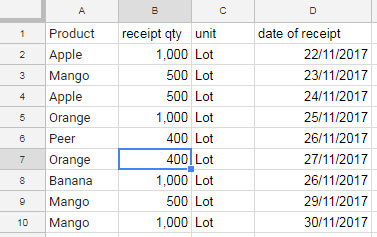
We can follow a simple sample data as below:

Example 1 with Numeric Criteria:
FILTER Function with Multiple Numeric Conditions or Criteria in Same Column.
Here I want to filter column B for received qty 400 or 500. Here is the filter formula to use.
=filter(A2:D, (B2:B = 400) + (B2:B = 500))
Example 2 with Text Criteria:
How to Use FILTER Function with Multiple Text Criteria in Same Column.
Suppose you want to filter Column A for Apple or Mango, how to apply these multiple conditions in that same column? See the formula.
=filter(A2:D, (A2:A = “Apple”) + (A2:A = “Mango”))
Example 3 with Date Criteria:
Multiple Date Conditions in Same Column Filtering in Google Sheets.
Similar: How to Use Date Criteria in Filter Function in Google Sheets
Let us see how to filter same column for different dates.
=filter(A2:D,(D2:D = date(2017,11,22)) + (D2:D = date(2017,11,27)))
The above three conditions are the most commonly used criteria type in Google Sheets Filter Function.
Conclusion
This way, you can use multiple conditions in same column filtering in Google Sheets. Hope to see you again with another awesome Google Doc spreadsheet tutorial. Enjoy!


=FILTER(Data!$A:$AN,Data!$P:$P ="",Data!$E:$E ="",Data!$U:$U ="",(Data!$G:$G "Deal Cancelled")+(Data!$G:$G ""&"")+(Data!$G:$G""&"Buyback"))Error Occurred anyone helps me to get resolved this formula.
Hi, Arvind Kumar,
You may please try either of the below Filter or Query formulas.
Filter;
=FILTER(Data!$A:$AN,Data!$P:$P ="",Data!$E:$E ="",Data!$U:$U ="",(Data!$G:$G= "Deal Cancelled")+(Data!$G:$G="")+(Data!$G:$G="Buyback"))Query;
=QUERY(Data!$A:$AN,"Select * where P is null and E is null and U is null and (G= 'Deal Cancelled' or G is null or G='Buyback')")If this is not working, please explain the problem instead of giving a non-working formula.
Thanks.
Thanks, this was really helpfull!