We can use a combination of BYROW, MIN, and SMALL with FILTER or XLOOKUP to lookup the smallest value in a 2D array in Google Sheets.

What Does It Mean to Lookup the Smallest Value in a 2D Array?

Assume you have sales dates in a column (range A2:A11) and sales quantities from different regions in the next few columns (B2:E11). The task is to find the first, second, and third smallest values from the range B2:E11 and return the corresponding dates from A2:A11.

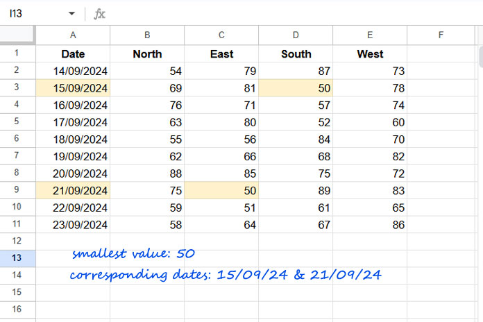
Yes—you want to lookup the smallest value in a 2D array in Google Sheets and return the matching date(s). That’s what we’re covering in this tutorial.

Step 1: Find the Smallest Value in a 2D Array

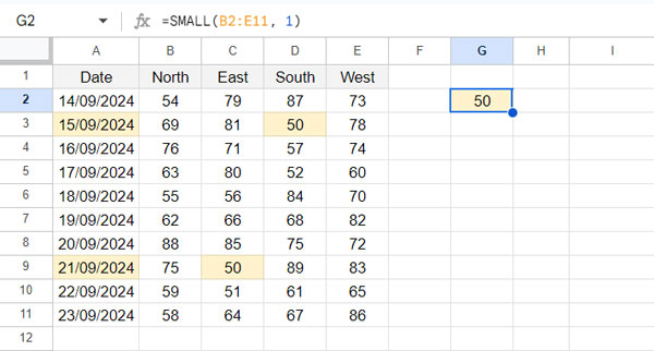
To find the smallest value in the range B2:E11, use the following formula:

=SMALL(B2:E11, 1)

Enter this in cell G2.

Finding the Nth Smallest Value in a 2D Array

To find the second smallest value, change 1 to 2. For the third smallest, use 3, and so on.

For this example, let’s find the smallest value in the 2D array. The formula returns 50. If you manually scan the range, you’ll find this value in cells D3 and C9.

Step 2: Match the Smallest Value in Each Row

Now we’ll compare the overall smallest value from the 2D array (from Step 1) with the smallest value in each row to identify which rows contain that value.

Use the following formula in H2 and drag it down to H11:

=$G$2=MIN(B2:E2)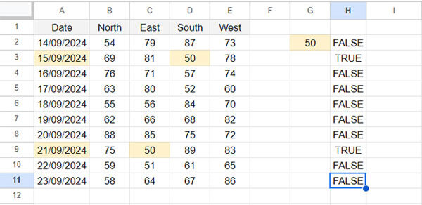

If the result is TRUE, it means that row contains the overall smallest value.

✅ Note:

• Use SMALL in Step 1 to find the nth smallest value in the entire 2D array.
• But in Step 2, since you’re only checking for the smallest value in each row, you can simply use MIN.

Step 3: Lookup the Smallest Value in a 2D Array (Using TRUE for Match)

To lookup the smallest value in a 2D array and return the date(s), use XLOOKUP or FILTER.

Option 1: XLOOKUP (Returns the First Match)

=XLOOKUP(TRUE, H2:H11, A2:A11)

This searches for TRUE in H2:H11 and returns the corresponding date from A2:A11.

👉 Example output: 15/09/2024

Option 2: FILTER (Returns All Matches)

=FILTER(A2:A11, H2:H11)

This returns all matching dates where the row contains the smallest value.

👉 Example output: 15/09/2024, 21/09/2024

Lookup the Smallest Value in a 2D Array with a Single Formula (No Helper Column)

Prefer a cleaner formula without using a helper column like H2:H11? You can combine BYROW, LAMBDA, MIN, and SMALL for that.

Here’s how:

BYROW(B2:E11, LAMBDA(r_range, SMALL(B2:E11, 1)=MIN(r_range)))

This checks each row to see if the row contains the overall smallest value in the array.

Now, plug that into XLOOKUP or FILTER:

XLOOKUP (Single Match)

=XLOOKUP(
   TRUE, 
   BYROW(B2:E11, LAMBDA(r_range, SMALL(B2:E11, 1)=MIN(r_range))), 
   A2:A11
)

FILTER (Multiple Matches)

=FILTER(
   A2:A11, 
   BYROW(B2:E11, LAMBDA(r_range, SMALL(B2:E11, 1)=MIN(r_range)))
)

Just replace 1 with 2, 3, or n if you want the nth smallest value.

Additional Tip: Lookup the Nth Unique Smallest Value in a 2D Array

We used SMALL(B2:E11, 1) to get the smallest value in the 2D array. But what if the smallest value repeats?

In our example, the first smallest value (50) appears multiple times. So using SMALL(..., 2) might still return 50.

To find distinct smallest values, use UNIQUE with TOCOL:

=SMALL(UNIQUE(TOCOL(B2:E11, 3)), 1)

• TOCOL(B2:E11, 3) flattens the 2D range into a single column.
• UNIQUE(...) removes duplicates.
• SMALL(..., n) returns the nth smallest unique value.

Use this in a cell like G2 if you’re using a step-by-step (non-array) approach.

To use this in the full array formula, just replace SMALL(B2:E11, 1) with:

SMALL(UNIQUE(TOCOL(B2:E11, 3)), 1)

This allows you to lookup the smallest value in a 2D array without duplicates.

Resources

• Index with Match for 2D Array Result in Google Sheets
• Row-Wise Sorting in a 2-D Array in Google Sheets
• How to Highlight the Smallest N Values in Each Row in Google Sheets
• Skip Duplicates in Min | Small Value Highlighting Row Wise in Google Sheets
• Average of Smallest N Values in Google Sheets (Zero and Non-Zero)