


 to a new value by applying a LAMBDA function.)
The MAP function in Google Sheets maps each value in an array(s) to a new value by applying a LAMBDA function.
As far as I know, it’s the one and only LAMBDA helper function (LHFs) in Google Sheets, which takes multiple arrays.
So obviously, it will take multiple name arguments within the LAMBDA.
For example, if you want to use three arrays individually in your MAP formula, you must specify name1, name2, and name3 within the LAMBDA.
The BYCOL, BYROW, SCAN, and REDUCE functions take a single array or range, whereas the MAKEARRAY takes only row and column numbers to create a calculated array.
MAP Function Syntax and Arguments in Google Sheets
Map Function Syntax:
MAP(array1, [array2, ...], LAMBDA)Where;
array1 – An array or range to be mapped.
array2, … – Additional arrays or ranges to be mapped.
LAMBDA – A LAMBDA function, contains ‘n’ name arguments matching the number of arrays, to map each value in the given arrays or ranges and to return new mapped value(s).
LAMBDA Syntax:
=LAMBDA([name, ...],formula_expression)(function_call, ...)Notes:-
- The highlighted part is not required. We should only use it when testing a LAMBDA formula in a cell. For more details, please check my Google Sheets function guide.
- We can read the syntax for the MAP function as
LAMBDA(name1, ..., formula_expression).
How to Use the MAP Function in Google Sheets
Without further ado, let’s go to an example. Please check the screenshot below to find two similar tables.
Table # 1 contains our sample data, and Table # 2 is our expected output (formula replaces 0 with blank).
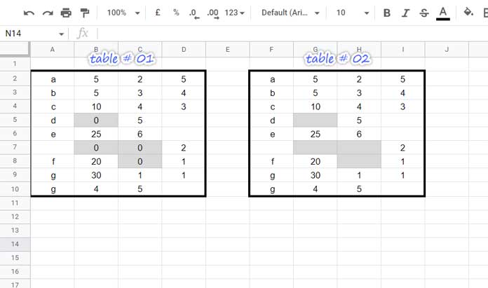
How to use the MAP function in Google Sheets to map each value in table # 1 and replace 0 with blank by applying a LAMBDA to each value?
Here are the step-by-step instructions to code a MAP formula in Google Sheets.
It involves three steps: a native or, we can say, regular Google Sheets formula > LAMBDA > MAP.
1. IF Logical Test (Regular Google Sheets Formula):
Insert the following IF formula in F2.
=if(A2=0,"",A2)2. Let’s convert it to a LAMBDA (the vivid Red highlighted part is not required in step # 3 below).
=lambda(v,if(v=0,"",v))(A2)3. Finally, convert it to a MAP formula.
=map(A2:D10,lambda(v,if(v=0,"",v)))In this formula, A2:D10 is the array, and v is the name1.
The formula uses only one name argument because it has only one array or range.
You May Also Like: Replace Blank Cells with 0 in Query Pivot in Google Sheets.
In the following examples, you will see the use of multiple arrays and names.
Examples
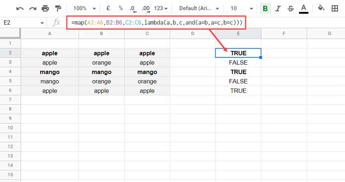
We can use the MAP function to expand logical tests involving AND, OR, and NOT to each row in an array.
For example, we can use the following formula to test whether all the values in A2:C2 are equal.
=and(A2=B2,A2=C2,B2=C2)But we won’t be able to expand it using the ArrayFormula function as below.
=ArrayFormula(and(A2:A6=B2:B6,A2:A6=C2:C6,B2:B6=C2:C6))I’ll walk you through how to use the MAP function in such scenarios.
As a side note, it’s not impossible without the MAP function. For example, we can use the below alternative formula to expand AND (above formula).
=ArrayFormula((A2:A6=B2:B6)*(A2:A6=C2:C6)*(B2:B6=C2:C6))Related:- How to Use OR Logical to Return Expanded Result in Google Sheets.
1. Lambda Helper Function to Expand Logical AND
Before coding the formula, we must find the number of arrays we want to use.
Here it’s 3, and they are A2:A6, B2:B6, and C2:C6.
So there must be three name arguments within the LAMBDA. In our above example, we have used only one.
This time also we will code the MAP formula in three steps.
1. AND logical test (The regular or native formula):
=and(A2=B2,A2=C2,B2=C2)2. LAMBDA:
=lambda(a,b,c,and(a=b,a=c,b=c))(A2,B2,C2)3. MAP Formula:
=map(A2:A6,B2:B6,C2:C6,lambda(a,b,c,and(a=b,a=c,b=c)))2. MAP with FILTER Function
In a Google Sheets file, I have a table containing the delivery details of landscaping materials for the next week.
The content of the table is as follows.
- A2:A – Item names
- B2:B – The location of delivery
- C2:C -The quantity to deliver.
How to filter the table if the items are either “Gravel 10-20 mm” or “Cobble Stone” in column A and the delivery location is “Location 1” in column B.
We can use the MAP function in Google Sheets for the logical test.
Then use it as the criteria within a FILTER.
=FILTER(A2:C,map(A2:A,B2:B,lambda(a,b,and(or(a="Gravel 10-20 mm",a="Cobble Stone"),b="Location 1"))))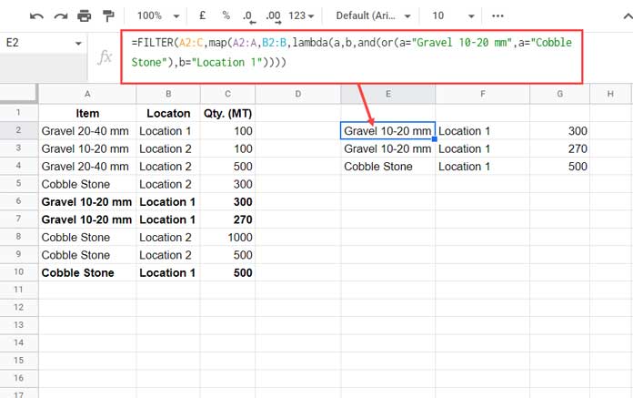
Do you want me to explain the above MAP and FILTER combination formula? If yes, please follow this.
Regular or ‘Native’ Logical Test:
=and(or(A2="Gravel 10-20 mm",A2="Cobble Stone"),B2="Location 1")We are converting it to a LAMBDA as earlier.
=lambda(a,b,and(or(a="Gravel 10-20 mm",a="Cobble Stone"),b="Location 1"))(A2,B2)The below MAP formula expands the output by taking array arguments.
=map(A2:A,B2:B,lambda(a,b,and(or(a="Gravel 10-20 mm",a="Cobble Stone"),b="Location 1")))The FILTER formula is as per the syntax =filter(range,map_formula_output=TRUE).
The =TRUE part is optional. So I’ve omitted that in my formula.