 in Google Sheets")

")

")


")


")


The ISTEXT function is one of the “Info” category functions in Google Sheets that help prevent or identify mixed data types.
The purpose of the ISTEXT function is to test a value and return TRUE if it’s text; otherwise, it returns FALSE.
You can use it in data validation to ensure data consistency and in conditional formatting to identify mixed data types. Additionally, you can use it in logical tests in formulas.
As a side note, you can avoid mixed data types in Google Sheets by converting your existing range to a table and choosing data types for each column.
Syntax of the ISTEXT Function in Google Sheets:
ISTEXT(value)Where value is the value to be verified.
Basic Formula Examples
=ISTEXT(100) // returns FALSE
=ISTEXT("InfoInspired") // returns TRUE
=ISTEXT(A1) // returns TRUE if A1 contains text, else FALSE
You can use ISTEXT in a range to verify each value in it by entering it as an array formula:
=ArrayFormula(ISTEXT(A2:A10))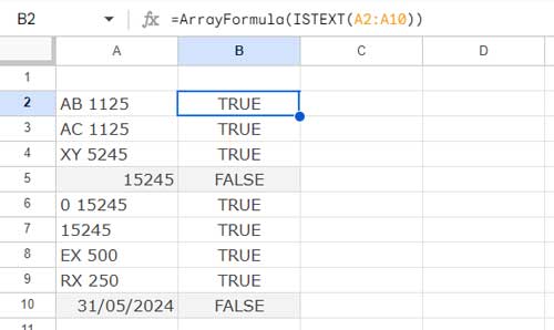
ISTEXT Function in Logical Tests
Example 1: To set an alert
You want to alert a user when they make an invalid entry. For example, if you expect an ID in cell B2, which should be text, the following formula in cell C2 will return “Please enter a valid ID” if the entered value is not text:
=IF(ISTEXT(B2), "", "Please enter a valid ID")Example 2: To test if all the values in a range are text
The following formulas will return the number of text values in the range C2:C10. If the result is 0, it means all values are non-text, such as dates, numbers, or times:
=ArrayFormula(COUNTIF(ISTEXT(C2:C10), TRUE))
=SUMPRODUCT((ISTEXT(C2:C10)))
These formulas will help you identify and count text values in the specified range.
ISTEXT Function in Data Validation
To prevent any entry other than text in a cell, for example, cell B2, you can use the following ISTEXT formula in Data Validation in Google Sheets:
=ISTEXT(B2)Steps:
- Click Data > Data Validation
- Then click the Add Rule button
- Under “Apply to Range,” enter B2 because you are setting the rule for cell B2. If you want to apply the rule to B2:B10, enter B2:B10.
- Under “Criteria,” select “Custom formula is” from the drop-down list
- Copy-paste the above formula
- Go through the “Advanced Options” and click “Done”.
This way, you can use the ISTEXT function in data validation to prevent non-text entries in a cell or cell range.
Note: To remove the data validation rule, navigate to the cell or any cell in the cell range and click on Data > Data Validation. Click the rule, then click the “Remove Rule” button.
ISTEXT Function in Conditional Formatting
Similarly to data validation, you can use the ISTEXT function in conditional formatting.
To highlight whether the entry in cell B2 is text, you can utilize the earlier formula, i.e., =ISTEXT(B2), within conditional formatting.
Steps:
- Click Format > Conditional Formatting
- Under “Apply to Range,” enter B2 or B2:B10 (the cell or cell range beginning from cell B2 that you want to highlight)
- Under “Format Rules,” select “Custom formula is”.
- Copy-paste the above formula.
- Select a formatting style and click “Done”.
Note: To remove the highlighting rule, navigate to the cell or any cell within the cell range and click on Format > Conditional Formatting. Hover your mouse pointer over the rule, then click the Trash can icon.
Resources
- How to Use ISREF Function in Google Sheets [Formula and Examples]
- How to Use the ISFORMULA Function in Google Sheets
- How to Use the ISERROR Function in Google Sheets
- Difference Between ISERR and ISNA Functions in Google Sheets
- Practical Use of ISBLANK Function in Google Sheets
- How to Use ISNONTEXT Function in Google Sheets [Practical Use]
- How to Use ISEVEN Function in Google Sheets [Formula Examples]
- ISDATE Function and Better Alternative in Google Sheets
- How to Use the ISLOGICAL Function in Google Sheets
- Google Sheets ISODD Function – Formula Examples
- The ISURL Function in Google Sheets
- How to Use the ISBETWEEN Function in Google Sheets