How to Use COUNTIF with UNIQUE in Google Sheets

COUNTIF with UNIQUE and COUNTUNIQUEIFS are two different concepts in Google Sheets. The former is used to summarize a table, while the latter is used to get a unique count after applying criteria.

For example, if a table contains tree names in one column and their heights in another column (A1:B), you can use COUNTUNIQUEIFS to get the number of unique trees with heights greater than 20 meters.

Tree Name	Height (in meters)
Eucalyptus	27
Maple	15
Pine	25
Redwood	30
Willow	12
Eucalyptus	25
Eucalyptus	24
Maple	14

=COUNTUNIQUEIFS(A1:A, B1:B, ">20") // returns 3

In the same table, you can use COUNTIF with UNIQUE to generate a summary report where the first column contains the unique tree names and the second column contains the count of each tree.

We’ll explore this technique in this tutorial.

Step 1: Using UNIQUE to Extract Unique Items

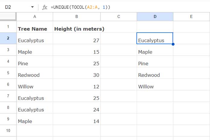
To extract the unique items (in this case, tree names) from A2:A, excluding the header row, use the following formula in cell D2:

=UNIQUE(TOCOL(A2:A, 1))

Extracting unique items for counting in Google Sheets

The TOCOL function removes empty rows from the range. If you don’t use this function, UNIQUE may return unique records along with a blank cell at the bottom, which can cause issues when we combine COUNTIF with UNIQUE.

Step 2: Counting the Unique Items with COUNTIF

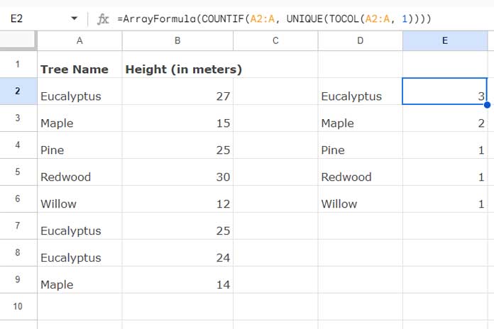
Enter the following COUNTIF array formula in cell E2 to count the unique items extracted:

=ArrayFormula(COUNTIF(A2:A, D2:D))

This will retain trailing zeros, which you might not be concerned about. However, the issue lies in using the extracted unique records range D2:D. To resolve this, simply replace D2:D with the formula from Step 1:

=ArrayFormula(COUNTIF(A2:A, UNIQUE(TOCOL(A2:A, 1))))

Example of using COUNTIF with UNIQUE in Google Sheets

The following two steps are optional.

Step 3: Combining COUNTIF with UNIQUE

In this step, we will combine both formulas to horizontally stack the counts with the unique values. We can use the HSTACK function with the following syntax:

HSTACK(range1, range2)

Here, range1 is the formula from Step 1, and range2 is the formula from Step 2:

=HSTACK(UNIQUE(TOCOL(A2:A, 1)), ArrayFormula(COUNTIF(A2:A, UNIQUE(TOCOL(A2:A, 1)))))

Remove the formulas in D2 and E2, and instead, enter this combined formula directly in cell D2.

Step 4: Simplifying COUNTIF with UNIQUE Using LET

The formula currently has repeated calculations, with the UNIQUE part appearing twice.

To simplify, we will assign the name ‘uni’ to the UNIQUE formula and ‘cnt’ to the COUNTIF formula using the LET function. Here’s the formula to be entered in cell D2:

=LET(uni, UNIQUE(TOCOL(A2:A, 1)), cnt, ArrayFormula(COUNTIF(A2:A, uni)), HSTACK(uni, cnt))

That’s how you can use COUNTIF with UNIQUE in Google Sheets.

QUERY as an Alternative Solution

If your data doesn’t contain mixed data types in a column (e.g., a column containing both numbers and text), you can use the QUERY formula as an alternative to the COUNTIF with UNIQUE formula.

You may get unexpected results when using a table with mixed data types in columns because QUERY might consider minority data types as null values.

In our sample data, there’s no such issue since the first column is text, and the second one is a number.

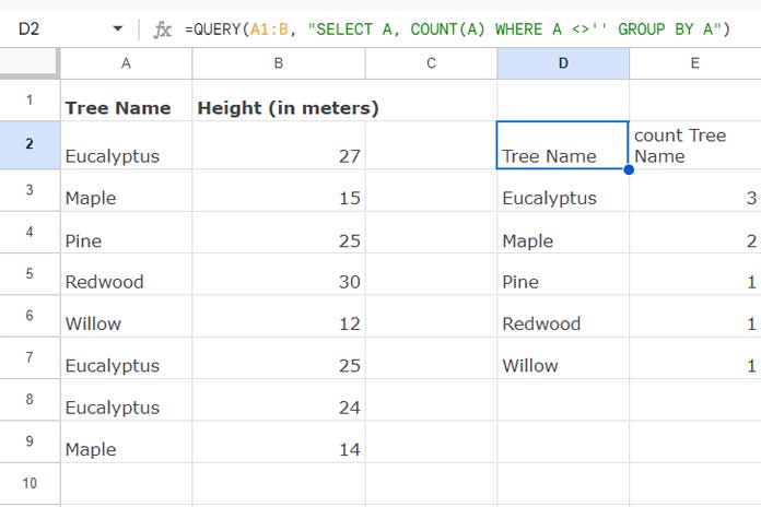
Here’s the QUERY formula:

=QUERY(A1:B, "SELECT A, COUNT(A) WHERE A <>'' GROUP BY A")

Using QUERY as an alternative to COUNTIF with UNIQUE in Google Sheets

Resources

17 COMMENTS

John Wolff December 15, 2022 At 4:55 am

Thank you so much! I wish I could have found this solution sooner!

Daniel Hanford September 8, 2021 At 2:59 am

Would there be a way of joining the name of the unique value and sum in a single cell with join( char(10))?

Results would be;

apples – 4
Oranges -2

- Prashanth September 8, 2021 At 11:06 am
  
  Hi, Daniel Hanford,
  
  We can achieve the count result as per your requirement.
  
  Assume the list in A2:A doesn’t contain a field label (header).
  
  =ArrayFormula(substitute(transpose(query(transpose(query(if(len(A2:A),A2:A&" -",), "Select Col1,count(Col1) where Col1 is not null group by Col1 label count(Col1)''")),,9^9)), "-",char(10)))
  
Hai Hoang September 7, 2021 At 3:01 pm

Thank you so much!!!

Hai Hoang September 7, 2021 At 10:51 am

Hello,

I have just found out about your wonderful blog.

I am working on Google Sheets, where people can create a list of items. I split those lists into separate cells.

That made me have a table where each item is stored in individual cells.

E.g.

row1: item 1 | item 2 | item 4
row2: item 4 | item 3 | item 1
row3: item 2 | item 1 | item 3

I would like to have a pie chart for counting the occurrence of items in all rows.

I am not sure if my answer is posted already somewhere. If so, please share the link.

Thank you so much

- Prashanth September 7, 2021 At 11:07 am
  
  Hi, Hai Hoang,
  
  Assume the values after the split is in the range A1:C.
  
  If so, make the columns F and G empty. Then insert the below Query formula in cell F1.
  
  =query(flatten(A1:C),"Select Col1,count(Col1) where Col1 is not null group by Col1 label count(Col1)''")
  
  Use that output to plot the Pie chart.
  
MaryAnn August 5, 2021 At 6:23 am

Hi! Is there a way to use the =COUNTA(UNIQUE formula to add a criterion, i.e., count unique text values if the amount is greater than x? Any suggestions would be wonderful! Thank you!!

- Prashanth August 6, 2021 At 2:06 pm
  
  Hi, MaryAnn,
  
  There is a specific function called COUNTUNIQUEIFS for this.
  
  =countuniqueifs(A2:A14,B2:B14,">5")
  It returns the count of unique texts in A2:A14 if corresponding numbers in B2:B14 are greater than 5.
  
  This Filter will also work.
  =counta(unique(filter(A2:A14,B2:B14>5)))
  
Ben Ponderin June 2, 2020 At 8:15 pm

Well done, Prashanth

Mark Leonard November 16, 2019 At 4:54 am

What if I want to count Multiple Unique Values depends on the time I input it.

Ex. If I input STA it will count 1 and if I input another STA below it will count 2 and so on.

STA 1
STA 2

Is this possible?

- Prashanth November 17, 2019 At 10:16 am
  
  https://infoinspired.com/google-docs/spreadsheet/running-count-in-google-sheets/
  
Hellen March 27, 2019 At 6:34 am

What if I need to count the unique values in one column / exclude duplicates, for example counting the number of individual students in column A? Is there a way to use Countif to do this?

- Prashanth March 27, 2019 At 9:16 am
  
  Hi, Hellen,
  
  For that, you can use Counta + Unique (if text string in column A) or Count+Unique (if numbers in column A).
  
  =COUNTA(unique(A1:A))
  
Viorel February 11, 2019 At 1:38 pm

Hey Prashanth,

Perfect. Thanks.

Cheers.

Viorel February 8, 2019 At 3:48 pm

What if I would need this to work based on 2 filters? For the above example, I would like to count unique names that were present (Y) on a specific date? What would the query be? Thanks.

- Prashanth February 9, 2019 At 9:06 am
  
  Hi,
  
  You can use this Query.
  
  =query(A1:C,"Select A, Count(A) where B=date '"&TEXT(E2,"yyyy-mm-dd")&"' and C='Y' group by A",1)
  
  In this formula, the cell E2 contains the criterion, i.e. the ‘specific date’.
  
  How to Use Date Criteria in Query Function in Google Sheets [Date in Where Clause]
  
  Best,
  
Adam July 30, 2018 At 11:24 pm

This worked perfectly and save me a ridiculous amount of time. Thanks so much for the thorough explanation of how to set Google Sheets like this!