In Google Sheets, you can use a custom highlight rule in conditional formatting to highlight all cells containing formulas.

If you prefer to see the formulas in the cells instead of highlighting them, there are two other methods available in the Edit and View menus.

In this tutorial, we will cover all options, including both highlighting and viewing methods.

Let’s start by applying a conditional formatting rule to highlight all cells with formulas in your sheets.

Steps to Highlight All Cells with Formulas

In the following example, I will apply a conditional formatting rule to highlight formulas in the range A1:F. I’ll also explain how to modify the steps for a different range or the entire sheet.

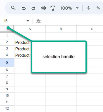
1. Select A1:F. If you want to highlight a different range, simply select it (to highlight the entire sheet, click the ‘selection handle’ in the top-left corner of the sheet, where the row and column headers intersect).
   
2. Go to the Format menu and click Conditional Formatting. This will open the “Conditional format rules” sidebar panel.
3. You’ll see your selected range under “Apply to Range.” You can modify it here if needed.
4. Select “Custom formula is” under “Format cells if.”
5. Enter =ISFORMULA(A1:F) (this should match the “Apply to range”) or =ISFORMULA(A1) (this should refer to the very first cell in the “Apply to range”). Both approaches will work.
6. Choose a fill color under Formatting Style.
7. Click Done.

This will highlight all cells that contain formulas in the selected range.

Some of you may want to find all cells containing formulas without using conditional formatting. There are two alternative approaches. Let me elaborate on that additional tip.

View All Cells Containing Formulas

To view all cells containing formulas, you can follow two approaches.

Method 1:

1. Click on View > Show > Formulas. This will reveal the formulas in the cells. To return to the previous state, click View > Show > Formulas again.

Method 2:

The second method uses the Find and Replace command.

1. Click Edit > Find and Replace.
2. In the “Find” field, enter =.
3. In the drop-down next to “Search,” select your option, preferably This Sheet.
4. Check Also search within formulas.

This will instantly show you the cells with formulas.

I suggest highlighting the cells with formulas, as this will make them easier to find.

Resources

• Highlight Filtered (Formula) Output in a Table in Google Sheets
• How to Highlight Cells Containing Special Characters in Google Sheets
• Google Sheets: Highlight If All The Cells Have Content in Range
• How to Highlight Cells Containing Specific Functions in Google Sheets
• Highlight Cells with Error Flags in the Drop-down in Google Sheets
• Highlight Text Only in Google Sheets