


After a quick succession of publishing two tutorials related to the financial functions in Sheets, I am back with a new tutorial. This time the topic is conditional formatting. Let me share with you how to highlight values in Sheet2 that match values in Sheet1 conditionally.
This is not just highlighting repeating values or duplicates. It involves condition too. So this post is about how to conditionally highlight duplicates in Google Sheets. But do remember. The list to compare for duplicates are in two tabs.
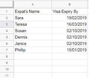
The first tab name “Sheet1” contains the below data.
Now here is the data in the tab name “Sheet2”. In this tab, I want the highlighting of the conditional match to be applied.
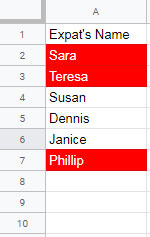
I want to highlight the names in this “Sheet2” tab, if the names match the below two criteria.
- The name must appear in column A in the tab “Sheet1”.
- The date (visa expiry) in column B against the name must be less than or equal to today.
For my example, I am using the above point # 2 as the condition. But you can use any other condition by slightly modifying the formula.
In the above screenshot, see the names in “Sheet2” highlighted. The reason the highlighted names are available in “Sheet1” also and the date in the next column to the name in Sheet1 is <= today.
How to Highlight Values in Sheet2 that Match Values in Sheet1 Conditionally in Sheets
If your conditional formatting of cells involves two or more tabs, you must use the INDIRECT function to refer to the second or third sheet.
Related: Role of Indirect Function in Conditional Formatting in Google Sheets.
For highlighting matching values between two sheets, we can use the COUNTIFS function. In this, we can use the INDIRECT to refer to “Sheet1”.
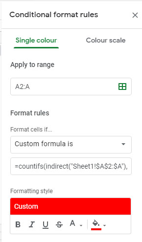
I am going to highlight the range A2:A in “Sheet2”. Here is the formula to highlight values in Sheet2 that match values in Sheet1 conditionally in Google Sheets.
=countifs(indirect("Sheet1!$A$2:$A"),$A2:$A,indirect("Sheet1!$B$2:$B"),"<="&today())If you have checked my earlier tutorial related to conditional formatting in Sheets, you may be already familiar with how to apply custom formula rules. So I am not going into the full detail here. Here is a quick walk thru’ instead.
To apply formatting rules in Google Sheets; Open the conditional formatting panel by clicking on the menu Format > Conditional formatting.
Follow the below settings there.
In the above example, I have a list of expat employees and their visa renewal dates in “Sheet1”.
From within “Sheet2”, we can check employee’s visa status, I mean whether it’s expired or renewed. If the name is highlighted, that means the visa of that particular employee has already expired.
In “Sheet2” you can use the expat’s names in different ways.
- If you want to check all the names, simply copy the names from “Sheet1” and paste it in “Sheet2” in the range A2:A.
- If you want to check the visa status of a few employees, just type their names in A2:A.
There is one more approach to conditionally highlighting values between sheets. That involves data validation drop-down.
Here is the detail.
Highlight Duplicate Value in Drop-Down If It’s Existing in a List in Another Tab
This is also simple. In cell A2 in “Sheet2”, create a drop-down menu. How?
- Go to Data > Data Validation.
- Select the “Criteria” as “List from Range”
- Enter the range “Sheet1!A2:A” in the given field and click “Save”
That’s all. The above custom formula will work here also. But for speed enhancements, do change the “Apply to range” to A2 in conditional format rules.
Additional Resources:
- How to Conditional Format Duplicates Across Sheet Tabs in Google Sheets.
- How to Highlight Cells Based on Expiry Date in Google Sheets.
- AND, OR, or NOT in Conditional Formatting in Google Sheets.
- How to Highlight Cells based on multiple Conditions in Google Sheets.
- Highlight Rows Based on Issue and Return of Items [Google Sheets].
- Highlight Duplicates in Single, Multiple Columns, All Cells in Google Sheets.
- Compare Two Google Sheets Cell by Cell and Highlight.
- Highlight Partial Matching Duplicates in Google Sheets.
- Highlight Visible Duplicates in Google Sheets.
Such an amazing tutorial.
Thank you so much, I see so many good things to learn here.