Highlighting rows based on issue and return status is a useful feature in Google Sheets for effective inventory tracking. Whether you’re managing a construction site or a library, this approach can help you easily monitor your inventory.

Why Highlight Rows by Issue and Return?

For inventory tracking, especially when dealing with multiple transactions, it’s essential to distinguish between items that are still checked out and those that have been returned.

This highlighting technique helps you quickly spot items that are still outstanding, which makes it easier to maintain an accurate inventory.

Understanding the Data Structure

If you record both issue and return transactions in the same row, you can easily identify missing return items.

However, if you log each transaction (issue or return) as a separate row, highlighting visually marks items still pending return.

Sample Data Setup

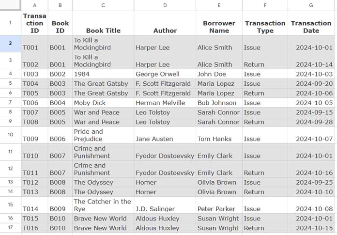
Let’s consider a library dataset with the following fields in cells range A1:G.

• Transaction ID: Unique identifier for each transaction
• Book ID: Identifier for each book
• Book Title: Title of the book
• Author: Author of the book
• Borrower Name: Name of the person borrowing the book
• Transaction Type: Either “Issue” or “Return”
• Transaction Date: Date of the transaction

For tracking, each unique entry needs identifiers such as Book ID, Borrower Name, and Transaction Type. If you’re working with other types of inventory, substitute the necessary fields (e.g., Item Code instead of Book ID).

You can make a copy of my sample dataset by clicking the button below.

Sample Sheet

Custom Formula for Highlighting Rows by Issue and Return Status

To highlight rows where the last transaction is a “Return,” we’ll use an XLOOKUP formula. This formula searches for each Book ID and Borrower Name combination from bottom to top, identifying the latest status of each item.

Formula:

=ArrayFormula(
   XLOOKUP($E2&$B2, $E$2:$E&$B$2:$B, $F$2:$F,, 0, -1)
)="Return"

Adjust the range in the formula to fit your dataset if it differs from the example.

Formula Breakdown:

• search_key: $E2&$B2 combines the Borrower Name and Book ID to create a unique identifier for each transaction.
• lookup_range: $E$2:$E&$B$2:$B creates a search range of combined Borrower Name and Book ID fields.
• result_range: $F$2:$F contains the Transaction Type (Issue or Return).
• missing_value: Omitted; if no match is found, an empty string is returned.
• match_mode: 0 for an exact match.
• search_mode: -1, which searches run from the bottom to the top, ensuring the formula finds the most recent transaction.

Logic: The formula retrieves the most recent transaction type for each item. If the last status is “Return,” the formula highlights the row, helping you easily identify items that are not currently checked out.

Applying the Highlighting Rule

Follow these steps to apply this custom rule in Google Sheets:

1. Select the range you want to highlight, e.g., A2:G.
2. Go to Format > Conditional Formatting.
3. Under Format rules, select Custom formula is.
4. Paste the XLOOKUP formula above into the formula field.
5. Choose your desired highlighting style in Formatting style.
6. Click Done.

This setup will highlight all rows where the last transaction for an item is “Return,” making it clear which items are still checked out.