


")


")

")
")
 in Excel & Google Sheets")


When working with time-based or continuously updated data in Google Sheets, you may want to highlight the last N values — for example, the most recent 10 days of sales, attendance, or performance scores.
Highlighting the last rows using conditional formatting makes it easier to spot trends and focus on the most relevant part of your dataset.
But before applying formulas, it’s important to clarify what “latest” means in your sheet. Does it refer to the most recent dates in a Date column, or simply the last N rows of data entered? The answer depends on how your data is structured.
How to Define the Latest N Values in Google Sheets
There are two common ways to define “latest” in Google Sheets:
1. Based on Dates (recommended)
If your dataset includes a Date column, “latest” refers to the values associated with the most recent dates.
Example: If column A has dates and column B has values, the “last 10 values” would be those tied to the 10 most recent dates.
This method ensures accuracy even if your data isn’t entered in order.
2. Based on Row Order
If your dataset doesn’t include dates, “latest” usually means the last N rows entered in the sheet.
Example: In B2:B95, highlighting the last 10 values would simply mean highlighting rows 86 to 95.
Use the date-based approach whenever a Date column exists, since it’s more reliable. The row-order method is useful only when dates aren’t available.
Highlight Last N Values Based on Dates
Assume the dates are in column A2:A and the values are in column B2:B. To highlight the latest 10 values, you can use the following custom formula in conditional formatting:
=XMATCH(A2, ARRAY_CONSTRAIN(SORT(FILTER($A$2:$A, $B$2:$B), 1, FALSE), 10, 1))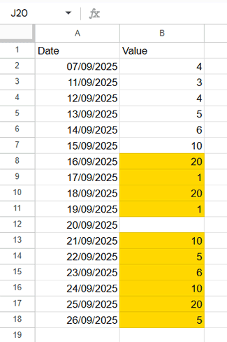
Why this works
- ✅ Skips empty cells (only highlights valid values)
- ✅ Doesn’t throw errors if there are fewer than N values
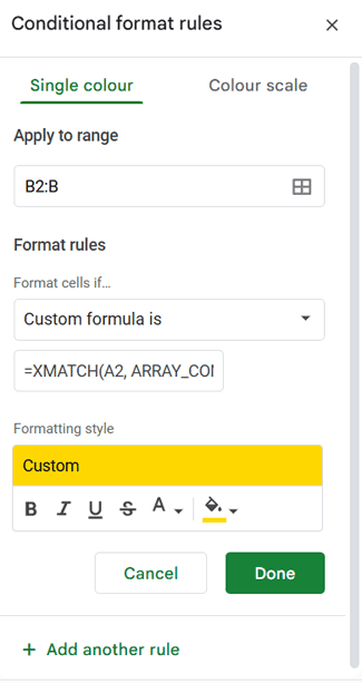
Steps to Apply Conditional Formatting
- Select the range
B2:B. - Go to Format > Conditional Formatting.
- Under Format rules, choose Custom formula.
- Enter the formula above.
- Pick a highlight color and click Done.
Formula Explanation
FILTER($A$2:$A, $B$2:$B)→ Filters dates where column B is not empty.SORT(..., 1, FALSE)→ Sorts the filtered dates in descending order (latest first).ARRAY_CONSTRAIN(..., 10, 1)→ Limits the result to 10 rows, 1 column (avoids errors when N is larger than the available values).XMATCH(A2, ...)→ Checks whether the current row’s date exists in the constrained array. If yes, the corresponding cell is highlighted.
This way, you can highlight the last N values by date in Google Sheets.
Highlight Last N Values Based on Row Order
If you don’t have a Date column, you can still highlight the last N rows. In this case, the bottom rows are treated as the most recent entries.
Use this formula in conditional formatting:
=XMATCH(ROW(A2), ARRAY_CONSTRAIN(SORT(FILTER(ROW($B$2:$B), $B$2:$B), 1, FALSE), 10, 1))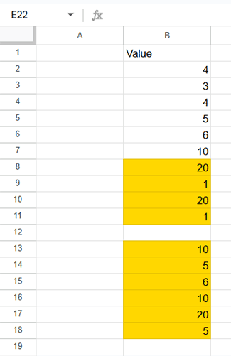
Why this works
- Uses row numbers instead of dates
- Skips empty rows
- Sorts row numbers in descending order
- Limits to the last N rows (in this example, 10)
This highlights the last N non-empty rows in your range.
Conclusion
Highlighting the last N values in Google Sheets can be done in two main ways:
- By dates → the most recent N values based on a Date column (recommended).
- By row order → the bottom N rows, when no Date column is available.
Both methods rely on custom formulas in conditional formatting, ensuring your Google Sheet always highlights the most recent values automatically.