Highlight the Latest Value or Status Change Rows in Google Sheets

In this tutorial, we’ll see how to use conditional formatting to highlight the latest value/status change rows in Google Sheets.

I have an employee database in Sheets that tracks job titles.

For example, take employee Ben:

He joined in January as an Engineer.
Later, in May, his designation changed to Manager.
After that, there were no more changes.

So the latest value change for Ben is in May. That’s the row I want to highlight.

I have already posted a tutorial on how to filter the last status change rows. You can check that here – Google Sheets: Show Only the Last Status Change per Name.

Here, instead of filtering, we’ll use highlighting.

Table of Contents

Sample Data

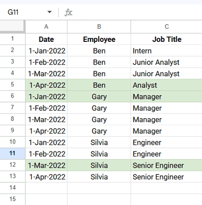
We have the following data in A1:C:

Date	Employee	Job Title
1-Jan-2022	Ben	Intern
1-Feb-2022	Ben	Junior Analyst
1-Mar-2022	Ben	Junior Analyst
1-Apr-2022	Ben	Analyst
1-Jan-2022	Gary	Manager
1-Feb-2022	Gary	Manager
1-Mar-2022	Gary	Manager
1-Apr-2022	Gary	Manager
1-Jan-2022	Silvia	Engineer
1-Feb-2022	Silvia	Engineer
1-Mar-2022	Silvia	Senior Engineer
1-Apr-2022	Silvia	Senior Engineer

Column C is where the values change.

👉 Important: Your data should be sorted first by Date, then by Employee.
This way, the formula can correctly identify the latest status change rows.

Ben: last change → 1-Apr-2022
Gary: no changes → highlight the first row (1-Jan-2022)
Silvia: last change → 1-Mar-2022

👉 Edge case: If an employee goes Engineer → Senior Engineer → Engineer, the formula will highlight the first Engineer row, not the last one. Rare case, but good to know.

Google Sheets Conditional Formatting Formula

We need a custom formula for this:

=AND(
  $B2<>"", 
  ROW($B2)=
    ARRAYFORMULA(
      XLOOKUP(
        $B2 & XLOOKUP($B2, $B$2:$B, $C$2:$C, , 0, -1), 
        $B$2:$B & $C$2:$C, 
        ROW($B$2:$B)
      )
    )
)

Highlight latest status change rows in Google Sheets with conditional formatting

In Google Sheets, this helps you track the date when each employee’s latest status change began.

Steps to Apply Conditional Formatting

Select your dataset (A2:C).
Go to Format → Conditional Formatting.
Under Format rules, pick Custom formula is.
Paste the above formula.
Choose a highlight color.
Done.

Now the latest change rows are highlighted automatically.

Formula Explanation

The inner XLOOKUP looks from bottom to top and fetches the latest job title for each employee.
The outer XLOOKUP returns the row number of that match.
ARRAYFORMULA is necessary here because we’re combining arrays (Employee&JobTitle) and need the formula to handle multiple rows at once.
AND($B2<>"", …) just avoids blank rows.

Example:
Take Silvia. Her job titles are:

Jan → Engineer
Feb → Engineer
Mar → Senior Engineer
Apr → Senior Engineer

The inner XLOOKUP (bottom-to-top) finds Senior Engineer as Silvia’s latest role.
The outer XLOOKUP (top-to-bottom) then returns the row number of the first occurrence of Senior Engineer for Silvia (i.e., the row on Mar 1).
That’s why the formula highlights Silvia’s Mar 1 record — her last status change.

So, the formula highlights the row where the last value change for each employee is recorded.

Sample Sheet

You can make a copy of the sample sheet I used in this tutorial.

Copy Sample Sheet

Note: The sheet also contains formulas from my previous tutorial on filtering the latest status change rows. You can safely ignore them while testing the highlighting rule.

Conclusion

Using conditional formatting with XLOOKUP, you can dynamically highlight the latest value or status change rows in Google Sheets, making it easier to track updates without filtering your data.

For more techniques like this, explore The Ultimate Guide to Conditional Formatting in Google Sheets, which includes 80+ tutorials covering everything from basic rules to advanced formula-driven formatting.