Highlight Duplicate Values Based on Occurrence Days in Google Sheets

Published on

This conditional format tutorial explains how to highlight duplicate values based on occurrence days in Google Sheets.

If you check the “Resources” at the end of this post, you can find a few tutorials that shed some light on basic conditional formatting related to duplicates.

But none of them address how to highlight duplicate values based on their occurrence days.

For example, I sold a couple of books online last year.

I have recorded the same in Google Sheets in two columns – date and book title columns.

How to highlight the books that are sold within 30 days from their last sale?

I am approaching this conditional formatting requirement from two different angles.

  1. Highlight all the duplicate values (books) based on their occurrence days.
  2. Highlight only the unique duplicate values (books) based on their occurrence days.

In the above second approach, a book once highlighted won’t be highlighted again. It is to avoid highlighting clutters.

Prerequisite (Sorting)

We must sort the table first.

We can sort the table in two different ways – 1) Sort by “Date” and then by “Title” or Sort by “Title” then by “Date.”

I am following the latter here. For that, please follow the below steps.

  • Select the range A1:B in which A1:A contains sold dates, and B1:B contains book titles (please scroll down and look at image # 2).
  • Go to Data > Sort range > Advanced range sorting options.
  • Check “Data has header rows.”
  • Sort by Title – A -> Z
  • Click on “Add another sort columns.”
  • Then by Date – A -> Z.
  • Click Sort.
Sorting Range for Conditional Formatting - Prerequisites
image # 1

Now let’s code the conditional format rule to highlight duplicate values based on occurrence days in Google Sheets.

Highlight UNIQUE Duplicate Values Based on Occurrence Days Less Than 30

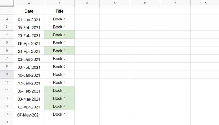
Assume I have sold “Book 1” on 01-Jan-2021, 05-Feb-2021, 25-Feb-2021, 06-Apr-2021, and 21-Apr-2021.

The number of days between 01-Jan-2021 and 05-Feb-2021 is 36 days. It’s above the limit, i.e., <=30 days.

So we should continue the check.

This time find the difference between 05-Feb-2021 and 25-Feb-2021, and we will get 21 days, i.e., within the limit.

So the formula must highlight the row that contains 25-Feb-2021.

We do not need to check further because we want to highlight unique duplicate values based on their occurrence days.

Here is the code to highlight unique duplicates based on occurrence days.

=and(
     len(A2),
     len(B2),
     A2=sortn(
        filter(
           {filter($A$2:$A,$B$2:$B=B2);"x"},
           {filter($A$2:$A,$B$2:$B=B2);"x"}-
           {"x";filter($A$2:$A,$B$2:$B=B2)}<31
        )
     )
)
Highlight Unique Duplicates Based on Occurrence Days
image # 2

I know there are several things to explain related to the above rule. Let’s start one by one.

We can apply the above rules in column A, Column B, or entire rows.

In my steps, I am just highlighting column B.

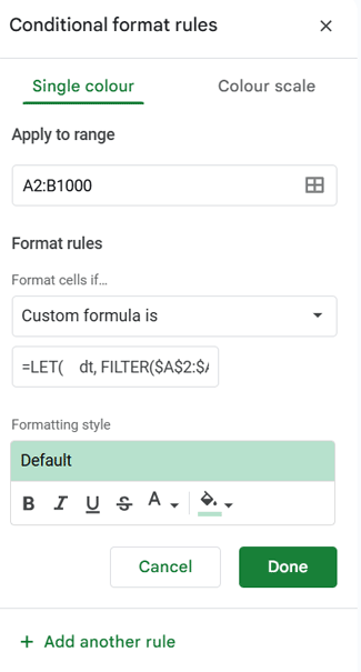
Here are the steps to apply the custom formula to highlight duplicate values based on occurrence days in Google Sheets.

  1. Copy the above formula.
  2. Select B2:B.
  3. Go to Format > Conditional formatting.
  4. Under “Format rules,” select “Custom formula…”
  5. Paste the above rule.
  6. Choose a color from the color palette under “Formatting style.”
  7. Click “Done.”

Highlight Rule Explanation

We have used the AND logical test to return TRUE (highlight) if all of the three provided arguments are logically true.

Syntax: AND(logical_expression1, logical_expression2, logical_expression3)

  1. len(A2) – A2 is not blank (logical_expression1)
  2. len(B2) – B2 is not blank (logical_expression2)
  3. Check whether the value is sold within 30 days of the last sale. This requires a detailed explanation, and here it is (logical_expression3).
A2=sortn(
        filter(
           {filter($A$2:$A,$B$2:$B=B2);"x"},
           {filter($A$2:$A,$B$2:$B=B2);"x"}-
           {"x";filter($A$2:$A,$B$2:$B=B2)}<31
        )
   )

There are four filters and a sort function.

What do the four FILTER formulas do in the above formula?

This illustration may help.

Highlight Duplicates Less Than N Days - Explained
image # 3

The above formula returns the dates 25-Feb-2021 and 21-Apr-2021 (highlighted in yellow color in the illustration above).

The role of SORTN here is to limit the output to 1 cell, i.e. 25-Feb-2021.

The custom formula rule actually tests whether A2=25-Feb-2021 in the first row.

Since the above is a conditional format rule, the logical testing will take place in each row.

The relative references in the formula, i.e., A2 and B2 will become A3, B3, A4, B4, and so on in each row.

How to Change Duplicate Entry Range from within 30 Days to 7 Days?

Please check for <31 in the formula. Modify that to <8.

That will highlight duplicate values based on seven days’ occurrence in Google Sheets.

Highlight ALL Duplicate Values Based on Occurrence Days Less Than 30

Here, you require to make two-three changes.

I’ll come to that later. Here is the formula rule and output.

=and(
     len(A2),
     len(B2),
     regexmatch(
        row(A2)&"",
        "^"&textjoin("$|^",true,
           filter(
              {filter(row($A$2:$A),$B$2:$B=B2);"x"},
              {filter($A$2:$A,$B$2:$B=B2);"x"}-
              {"x";filter($A$2:$A,$B$2:$B=B2)}<31)
           )
        &"$"
     )
)
Highlight All Duplicates Based on Occurrence Days
image # 4

In the earlier example, I have explained why the formula highlights “Book 1” in cell B4.

Here the formula also highlights the “Book 1” in cell B6.

It’s because the number of days between the dates in B6 and B5 is also less than 30 days.

I have made a few changes here.

Removed the Sortn function that limits the output to one value because we wish to highlight all duplicates based on occurrence days.

In the outer filter, instead of filtering dates, I have used the ROW function to filter rows.

So the output won’t be 25-Feb-2021 and 21-Apr-2021 (please refer to image # 3); instead, corresponding row numbers.

The REGEXMATCH matches the row numbers and highlights cells accordingly.

Note:- The TEXTJOIN combines the returned row numbers to form a regular expression in Regexmatch.

That’s all about how to highlight duplicate values based on occurrence days in Google Sheets.

Thanks for the stay. Enjoy!

Resources

Prashanth KV
Prashanth KV
Your Trusted Google Sheets and Excel Guide Prashanth KV brings a wealth of experience in Google Sheets and Excel, cultivated through years of work with multinational corporations in Mumbai and Dubai. As a recognized Google Product Expert in Docs Editors, Prashanth shares his expertise through insightful blogging since 2012. Explore his blog for practical tips and guidance on maximizing your spreadsheet skills.

How to Extract Numbers from Text in Excel with Regex

You can use the REGEXEXTRACT or REGEXREPLACE functions to easily extract numbers from text...

Using OFFSET and MATCH Together in Google Sheets: Advanced Tips

One powerful and flexible way to look up values is by combining the OFFSET...

How to Use OFFSET and XMATCH Functions Together in Excel

We often use the OFFSET and XMATCH functions together to match a value in...

How to Calculate Maximum Drawdown in Excel and Google Sheets

You can use the following dynamic array formula to calculate maximum drawdown (MDD) in...

More like this

Using OFFSET and MATCH Together in Google Sheets: Advanced Tips

One powerful and flexible way to look up values is by combining the OFFSET...

Running Count with Structured References in Google Sheets

Running a count with structured references is achievable in Google Sheets tables using the...

Running Total with Structured Table References in Google Sheets

You can use two types of formulas to create a running total with structured...

LEAVE A REPLY

Please enter your comment!
Please enter your name here

This site uses Akismet to reduce spam. Learn how your comment data is processed.